Data Fitting#
Millikan: A Direct Photoelectric Determination of Planck’s \(h\)#
In 1914, Robert A. Millikan’s highly accurate measurements of the Planck constant from the photoelectric effect supported Einstein’s model, even though a corpuscular theory of light was for Millikan, at the time, “quite unthinkable”. Einstein was awarded the 1921 Nobel Prize in Physics for “his discovery of the law of the photoelectric effect”, and Millikan was awarded the Nobel Prize in 1923 for “his work on the elementary charge of electricity and on the photoelectric effect”. Source: Photoelectric Effect


Millikan, Physical Review 7 (3): 355-388 (1915)
import numpy as np
import matplotlib.pylab as plt
# import constants from scipy
import scipy.constants as cnst

# Milikan's data in wavelength (lambda) and volts
lamb, volts = np.loadtxt('./data/05_millikan.dat', unpack=True)

# get frequency from wavelength
freq = cnst.c / ( 1e-10 * lamb )

# plot data as Milikan did
plt.figure(1)
plt.grid(True)

plt.plot(freq, volts, 'o')

plt.xlabel('frequency (Hz)')
plt.ylabel('stopping voltage (V)')

plt.show()
---------------------------------------------------------------------------
FileNotFoundError                         Traceback (most recent call last)
Cell In[2], line 5
      2 import scipy.constants as cnst
      4 # Milikan's data in wavelength (lambda) and volts
----> 5 lamb, volts = np.loadtxt('./data/05_millikan.dat', unpack=True)
      7 # get frequency from wavelength
      8 freq = cnst.c / ( 1e-10 * lamb )

File /usr/local/lib/python3.14/site-packages/numpy/lib/_npyio_impl.py:1397, in loadtxt(fname, dtype, comments, delimiter, converters, skiprows, usecols, unpack, ndmin, encoding, max_rows, quotechar, like)
   1394 if isinstance(delimiter, bytes):
   1395     delimiter = delimiter.decode('latin1')
-> 1397 arr = _read(fname, dtype=dtype, comment=comment, delimiter=delimiter,
   1398             converters=converters, skiplines=skiprows, usecols=usecols,
   1399             unpack=unpack, ndmin=ndmin, encoding=encoding,
   1400             max_rows=max_rows, quote=quotechar)
   1402 return arr

File /usr/local/lib/python3.14/site-packages/numpy/lib/_npyio_impl.py:1024, in _read(fname, delimiter, comment, quote, imaginary_unit, usecols, skiplines, max_rows, converters, ndmin, unpack, dtype, encoding)
   1022     fname = os.fspath(fname)
   1023 if isinstance(fname, str):
-> 1024     fh = np.lib._datasource.open(fname, 'rt', encoding=encoding)
   1025     if encoding is None:
   1026         encoding = getattr(fh, 'encoding', 'latin1')

File /usr/local/lib/python3.14/site-packages/numpy/lib/_datasource.py:192, in open(path, mode, destpath, encoding, newline)
    155 """
    156 Open `path` with `mode` and return the file object.
    157
   (...)    188
    189 """
    191 ds = DataSource(destpath)
--> 192 return ds.open(path, mode, encoding=encoding, newline=newline)

File /usr/local/lib/python3.14/site-packages/numpy/lib/_datasource.py:529, in DataSource.open(self, path, mode, encoding, newline)
    526     return _file_openers[ext](found, mode=mode,
    527                               encoding=encoding, newline=newline)
    528 else:
--> 529     raise FileNotFoundError(f"{path} not found.")

FileNotFoundError: ./data/05_millikan.dat not found.
Simple / Polynomial Fits#
# use Numpy's polyfit
# ... degree = 1 yields: f(x) = a * x + b
# ... degree = 2 yields: f(x) = a * x^2 + b * x^1 + c * x^0
# ...

myFit = np.polyfit(freq, volts, deg=1)

print( " a =", myFit[0] )
print( " b =", myFit[1] )
 a = 3.9637242014216225e-15
 b = -4.25565315042055
# plot data as Milikan did ... with the fit
plt.figure(1)
plt.grid(True)

plt.plot(freq, volts, 'o')

#plt.plot(freq, myFit[0]*freq + myFit[1]) # a * x + b

plt.plot(freq, np.polyval(myFit, freq) )

plt.xlabel('frequency (Hz)')
plt.ylabel('stopping voltage (V)')

plt.show()
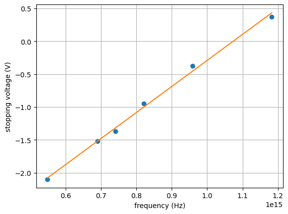
# compare fit to Scipy's value
h = cnst.e * myFit[0]
print('h_Millikan =', h, "Js")
print('h_Scipy    =', cnst.h, "Js")
h_Millikan = 6.3505862991380325e-34 Js
h_Scipy    = 6.62607015e-34 Js
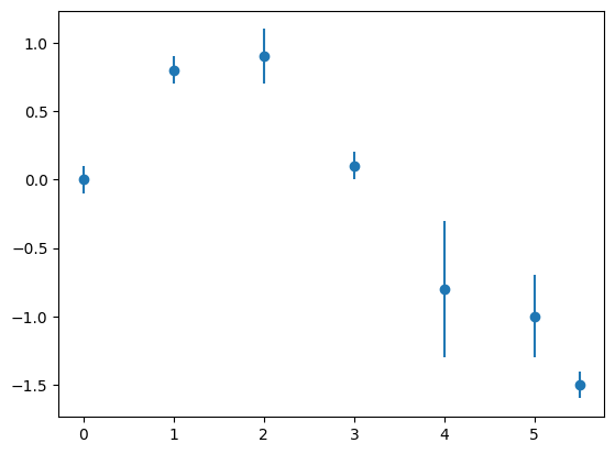
Polynomial Fits with Uncertain Data#
# data points and uncertainties
x     = np.array([0.0, 1.0, 2.0, 3.0,  4.0,  5.0,  5.5])
y     = np.array([0.0, 0.8, 0.9, 0.1, -0.8, -1.0, -1.5])
sigma = np.array([0.1, 0.1, 0.2, 0.1,  0.5,  0.3,  0.1])

# plot it
plt.figure(1)
plt.errorbar(x, y, sigma, fmt='o')
plt.show()
# define weights for each data point using sigma
weights = 1.0 / sigma**2.0

# do polynomial fit using weights
myFit, V = np.polyfit(x, y,
                      deg=4,
                      w=weights,
                      cov='unscaled') # get covariance matrix

print( myFit )
print( V )

# plot it
plt.figure(1)

p = np.poly1d(myFit)

xPlot = np.linspace(0, 5.5, 100)

plt.errorbar(x, y, sigma, fmt='o')

plt.plot(xPlot, p(xPlot), '-')

plt.show()
[-7.34798866e-04  6.52969070e-02 -6.37435606e-01  1.38085675e+00
 -1.43255678e-03]
[[ 1.21538331e-05 -1.16182064e-04  3.10235045e-04 -2.13832101e-04
   1.86834500e-06]
 [-1.16182064e-04  1.11264482e-03 -2.98218875e-03  2.07526380e-03
  -2.37965165e-05]
 [ 3.10235045e-04 -2.98218875e-03  8.05673097e-03 -5.72655652e-03
   1.04127651e-04]
 [-2.13832101e-04  2.07526380e-03 -5.72655652e-03  4.32307766e-03
  -1.81857695e-04]
 [ 1.86834500e-06 -2.37965165e-05  1.04127651e-04 -1.81857695e-04
   9.99389313e-05]]
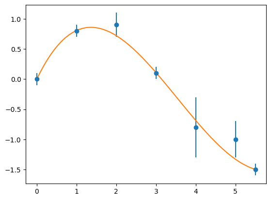
Calculate the difference between the original data and the fitted one by evaluating the polynomial using fitting parameters myFit and NumPy’s polyval function:
diffs = np.polyval(myFit, x) - y

# estimate the quality of the fit via chi^2:
#
#          chi^2 = Sum_i [Fit(x_i) - y_i]^2 / sigma_i^2.0
#  reduced chi^2 = chi^2 / (#x - #degree)
#

chi_squared = np.sum(diffs**2.0 / sigma**2.0)

red_chi_sq = chi_squared/(len(x) - 3)

print('    Chi sq =', chi_squared)
print('red Chi sq =', red_chi_sq)

# print out all fitting parameter and their "errors"
for ii in range(0, np.size(myFit)):

    myError = np.sqrt(V[ii,ii])

    print("       c_%d = %+f +/- %f"%(ii, myFit[ii], myError))
    Chi sq = 2.073762429982544
red Chi sq = 0.518440607495636
       c_0 = -0.000735 +/- 0.003486
       c_1 = +0.065297 +/- 0.033356
       c_2 = -0.637436 +/- 0.089759
       c_3 = +1.380857 +/- 0.065750
       c_4 = -0.001433 +/- 0.009997
Non-Linear Fits#
Example 1: Higher-order Polynomial Fit#
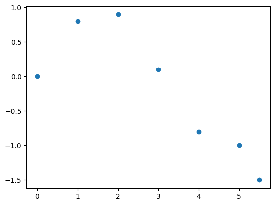
# define some test data ...
x = np.array([0.0, 1.0, 2.0, 3.0,  4.0,  5.0, 5.5])
y = np.array([0.0, 0.8, 0.9, 0.1, -0.8, -1.0, -1.5])

plt.figure(1)
plt.plot(x, y, 'o')
plt.show()
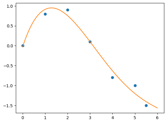
Fit it with an higher order polynom:
myFit = np.polyfit(x, y, deg=4)
print( myFit )
[-0.00765278 0.14641278 -0.93518463 1.7371271 -0.02772485]
# create a callable function from myFit (parameters)
myFitPolynom = np.poly1d( myFit )

# plot it on a self-defined grid
xPlot = np.linspace(0, 6, 100)

plt.figure(1)

# original data
plt.plot(x, y, 'o')

# fitted data
plt.plot(xPlot, myFitPolynom(xPlot), '-')

plt.show()
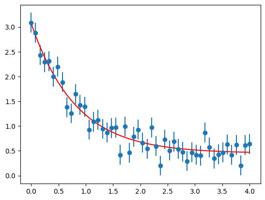
Example 2: Self-defined Fitting Function#
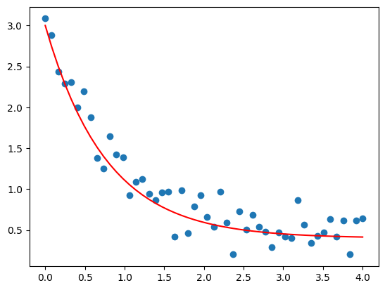
# load data including inaccuracies from file
xdata, ydata, sigma = np.loadtxt('./data/03_xyerr.dat').transpose()

plt.figure(1)

# and plot it
plt.plot(xdata, ydata, 'o')

# let's try to fit by hand
# ... using a scaled and shifted exp(-x) function

def myFitFunc(x, a, b, c):
    return a * np.exp(-b * x) + c

xFit = np.linspace(0, 4, 50)

yFit = myFitFunc(xdata, a=2.6, b=1.3, c=0.4)

plt.plot(xFit, yFit, 'r-')

plt.show()
Use Scipy’s curve_fit() function:
from scipy.optimize import curve_fit

def myFitFunc(x, a, b, c):
    return a * np.exp(-b * x) + c

myFit, V = curve_fit(myFitFunc,
                     xdata,
                     ydata,
                     sigma=sigma)

print( myFit )
print( V )
[2.62100319 1.22255364 0.44981714]
[[ 0.01107066  0.00384071 -0.0007366 ]
 [ 0.00384071  0.01219645  0.00421007]
 [-0.0007366   0.00421007  0.00254324]]
# print out all fitting parameter and their "errors"
chars = ['a', 'b', 'c']

for ii in range(0, np.size(myFit)):
    myError = np.sqrt(V[ii,ii])
    print("         %s = %+f +/- %f"%(chars[ii], myFit[ii], myError))
         a = +2.621003 +/- 0.105217
         b = +1.222554 +/- 0.110438
         c = +0.449817 +/- 0.050431
# evaluate fit function at original x-values

yFit = myFitFunc(xdata, *myFit)         # Note the usage of *myFit

# and get red chi^2 from this
red_chi_sq = np.sum((yFit - ydata)**2/sigma**2)/(len(xdata) - len(myFit))

print('red Chi sq =', red_chi_sq)
red Chi sq = 0.8233031279118471
# plot data including error bars
plt.errorbar(xdata, ydata, yerr = sigma, fmt = 'o')

# as well as the fit
plt.plot(xdata, yFit, 'r-')

plt.show()