Ordinary Differential Equations#
import numpy as np
import matplotlib.pyplot as plt
Solving ODEs using Euler’s Method#
\[
\large
\begin{align*}
& & \frac{\partial y(x)}{\partial x} &= F(x, y(x))
\end{align*}
\]
\[\begin{split}
\begin{align*}
\text{discretised:}& & \frac{\partial y(x_i)}{\partial x_i} &= F(x_i, y(x_i)) \\
\text{approximated:}& & \frac{y(x_{i+1}) - y(x_i)}{\Delta x} &\approx F(x_i, y(x_i)) \\
\end{align*}
\end{split}\]
\[
\large
\begin{align*}
\Rightarrow y(x_{i+1}) &\approx F(x_i, y(x_i)) \, \Delta x + y(x_i)
\end{align*}
\]
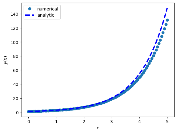
1. Example: \(y'(x) = y\)#
\[\begin{split}
\begin{align*}
\frac{\partial y(x)}{\partial x} &= y(x)
\quad \Rightarrow \quad y(x) = e^x + b \\
y(0) &= 1 \quad \Rightarrow \quad y(x) = e^x
\end{align*}
\end{split}\]
N = 100
x = np.linspace(0, 5, N)
y = np.empty(N)
dx = x[1] - x[0]

y[0] = 1    # initial value

def F(x, y):
    return y

# integrate "by hand"
for i in range(N-1):

    y[i+1] = y[i] + dx * F(x[i], y[i])

# plot it
plt.figure(1)
plt.plot(x, y, 'o', label='numerical')
plt.plot(x, np.exp(x), "b--", lw=3, label='analytic')
plt.xlabel('$x$')
plt.ylabel('$y(x)$')
plt.legend()

plt.show()
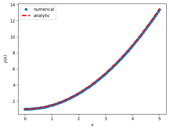
2. Example: \(y'(x) = x\)#
\[\begin{split}
\begin{align*}
\frac{\partial y(x)}{\partial x} &= x
\quad \Leftrightarrow y(x) = \int x \, dx \quad = \frac{1}{2} x^2 + b \\
y(0) &= 1
\quad \Rightarrow \quad y(x) = \frac{1}{2} x^2 + 1
\end{align*}
\end{split}\]
N = 100
x = np.linspace(0, 5, N)
y = np.empty(N)
dx = x[1] - x[0]

y[0] = 1    # initial value

def F(x, y):
    return x

for i in range(N-1):
    y[i+1] = y[i] + dx * F(x[i], y[i])

plt.figure(1)
plt.plot(x, y, 'o', lw=3, label='numerical')
plt.plot(x, 0.5 * x**2.0 + 1, "r--", lw=3, label='analytic')
plt.xlabel('$x$')
plt.ylabel('$y(x)$')
plt.legend()

plt.show()
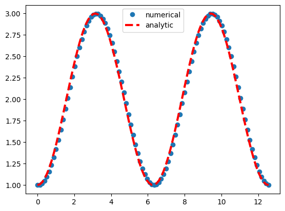
3. Example: \(y'(x) = sin(x)\)#
\[\begin{split}
\begin{align*}
\frac{\partial y(x)}{\partial x} &= sin(x)
&\quad \Rightarrow \quad y(x) &= -cos(x) + b \\
y(0) &= 1
&\quad \Rightarrow \quad y(x) &= -cos(x) + 2
\end{align*}
\end{split}\]
N = 100
x = np.linspace(0, 4*np.pi, N)
y = np.empty(N)
dx = x[1] - x[0]

y[0] = 1    # initial value

def F(x, y):
    return np.sin(x)

for i in range(N-1):
    y[i+1] = y[i] + dx * F(x[i], y[i])

plt.figure(1)
plt.plot(x, y, 'o', lw=3, label='numerical')
plt.plot(x, -np.cos(x) + 2, "r--", lw=3, label='analytic')
plt.legend()
plt.show()
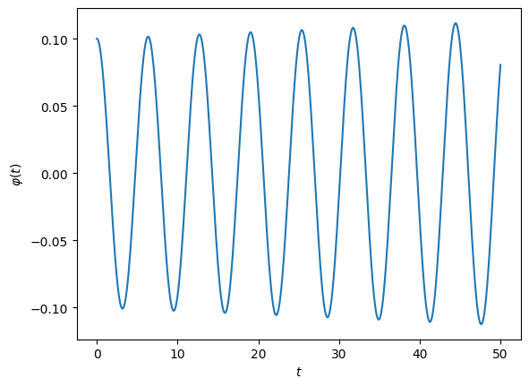
4. Example: Pendulum#

Second-oder ODE for the angle \(\varphi\):
\[\large \frac{\partial^2 \varphi}{\partial t^2} = - \frac{g}{l} \sin{\varphi}\]
Coupled system of first-order ODEs:
\[\begin{split} \large \begin{pmatrix}
\dot{\varphi} \\ \dot{\omega}
\end{pmatrix}
=
\begin{pmatrix} \omega \\ - \frac{g}{l} \sin{\varphi} \end{pmatrix}
\end{split}\]
N = 10000
g = 9.81    # m / s^2
l = 10.0    # m

time  = np.linspace(0, 50, N)
phi   = np.zeros(N)
omega = np.zeros(N)
dt    = time[1] - time[0]

phi[0]   = 0.1    # initial values
omega[0] = 0.0

def F(time, phi, omega):
    return [omega,
            -(g/l) * np.sin(phi)]

for i in range(N-1):

    phi[i+1]   = phi[i]   + dt * F(time[i],
                                   phi[i],
                                   omega[i])[0]

    omega[i+1] = omega[i] + dt * F(time[i],
                                   phi[i],
                                   omega[i])[1]

plt.figure(1)
plt.plot(time, phi)
plt.xlabel('$t$')
plt.ylabel('$\\varphi(t)$')
plt.show()
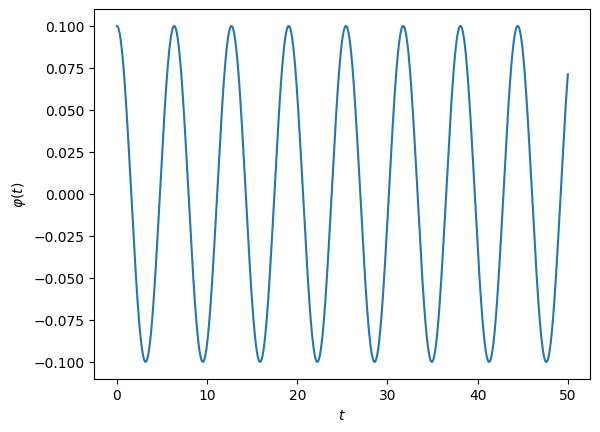
Solving ODEs using Predictor-Corrector Method#

N = 1000
g = 9.8
l = 10.0

time  = np.linspace(0, 50, N)
phi   = np.zeros(N)
omega = np.zeros(N)
dt    = time[1] - time[0]

phi[0]   = 0.1    # initial values
omega[0] = 0.0

def F(time, phi, omega):
    return [omega,
            -(g/l) * np.sin(phi)]

for i in range(N-1):

    phi_mid   = phi[i]   + 0.5*dt * F(time[i],
                                      phi[i],
                                      omega[i])[0]

    omega_mid = omega[i] + 0.5*dt * F(time[i],
                                      phi[i],
                                      omega[i])[1]

    phi[i+1]   = phi[i]   + dt * F(time[i],
                                   phi_mid,
                                   omega_mid)[0]

    omega[i+1] = omega[i] + dt * F(time[i],
                                   phi_mid,
                                   omega_mid)[1]

plt.figure(1)
plt.plot(time, phi)
plt.xlabel('$t$')
plt.ylabel('$\\varphi(t)$')
plt.show()
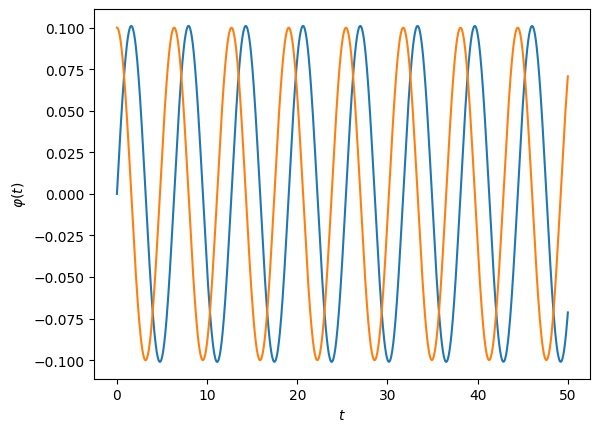
Solving ODEs using SciPy’s Runge-Kutta Method integrate.solve_ivp()#
1. Example: Pendulum – done right#
\[\begin{split}
\large
\begin{align*}
\begin{pmatrix} \dot{\varphi} \\ \dot{\omega} \end{pmatrix}
& = \begin{pmatrix} \omega \\ - \frac{g}{l} \sin{\varphi} \end{pmatrix}
\end{align*}
\end{split}\]
needs to be reacast into the following form:
\[\begin{split}
\large
\begin{align*}
\frac{\partial \vec{y}(t)}{\partial t} &= \vec{F}(t, \vec{y}(t))\\
\vec{y}(t) &= \begin{pmatrix} y_0(t) \\ y_1(t) \end{pmatrix} = \begin{pmatrix} \varphi(t) \\ \omega(t) \end{pmatrix} \\
\vec{F}_\text{Pendulum}(t, \vec{y}) &= \begin{pmatrix} y_1(t) \\ -\frac{g}{l} \sin{y_0(t)} \end{pmatrix}
\end{align*}
\end{split}\]
import scipy.integrate as integrate
N = 1000
g = 9.8
l = 10.0

tMin = 0
tMax = 50
time = np.linspace(tMin, tMax, N)

y_init = [0, 0.1]    # initial values

def FPendulum(t, y):
    F    = np.zeros(2)
    F[0] = y[1]
    F[1] = -(g/l) * np.sin(y[0])
    return F

sol = integrate.solve_ivp(FPendulum,
                          (tMin, tMax),
                          y_init, t_eval=time)

print(sol)
  message: The solver successfully reached the end of the integration interval.
  success: True
   status: 0
        t: [ 0.000e+00  5.005e-02 ...  4.995e+01  5.000e+01]
        y: [[ 0.000e+00  5.003e-03 ... -7.478e-02 -7.133e-02]
            [ 1.000e-01  9.988e-02 ...  6.715e-02  7.074e-02]]
      sol: None
 t_events: None
 y_events: None
     nfev: 326
     njev: 0
      nlu: 0
plt.figure(1)

plt.plot(sol.t, sol.y[0])
plt.plot(sol.t, sol.y[1])

plt.xlabel('$t$')
plt.ylabel('$\\varphi(t)$')
plt.show()
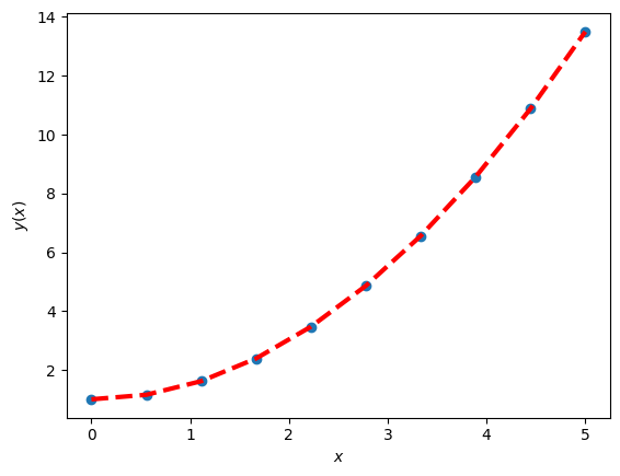
2. Example: \(y'(x) = x\)#
\[\begin{split}
\begin{align*}
\frac{\partial y(x)}{\partial x} &= x
\quad \Leftrightarrow y(x) = \int x \, dx \quad = \frac{1}{2} x^2 + b \\
y(0) &= 1
\quad \Rightarrow \quad y(x) = \frac{1}{2} x^2 + 1
\end{align*}
\end{split}\]
N = 10
x = np.linspace(0, 5, N)
y = np.empty(N)
dx = x[1] - x[0]

y0 = [1]    # initial value

def F(x, y):
    return x

sol = integrate.solve_ivp(F, (0, 5), y0, t_eval=x)

plt.figure(1)
plt.plot(x, sol.y[0, :], 'o', lw=3)
plt.plot(x, 0.5 * x**2.0 + 1, "r--", lw=3)
plt.xlabel('$x$')
plt.ylabel('$y(x)$')

plt.show()
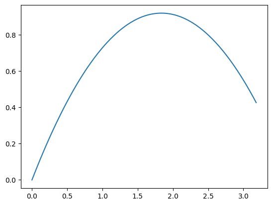
3. Example: Projectile motion#

g     = 9.8
v0    = 6.0
alpha = 45.0 / 180.0 * np.pi

N    = 200
tMin = 0
tMax = 0.75
time = np.linspace(tMin, tMax, N)

y0 = [0, 0]    # initial values

def FProjectile(t, y):

    F    = np.zeros(2)
    F[0] =  v0 * np.cos(alpha)
    F[1] =  v0 * np.sin(alpha) - g*t

    return F

sol = integrate.solve_ivp(FProjectile,
                          (tMin, tMax),
                          y0, t_eval=time)

plt.figure(1)

plt.plot(sol.y[0, :], sol.y[1, :])


#plt.ylim([0, 0.21])
#plt.xlim([0, 0.15])
plt.show()
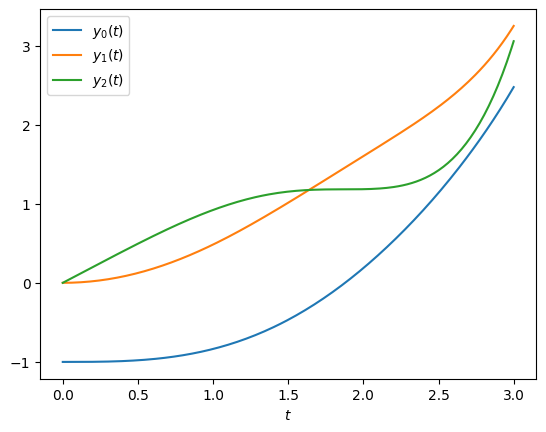
3. Example: Multidimensional#
\[\begin{split}
\begin{align*}
\frac{\partial \vec{y}(t)}{\partial t} = \vec{F}(t, \vec{y}) = \begin{pmatrix} y_1 \\ y_2 \\ y_0^2 \end{pmatrix}
\end{align*}
\end{split}\]
def F(t, y):
    myF    = np.zeros(3)
    myF[0] = y[1]
    myF[1] = y[2]
    myF[2] = y[0]**2.0
    return myF

N    = 200
tMin = 0
tMax = 3.0
time = np.linspace(tMin, tMax, N)

y0 = [-1, 0, 0]   # initial values

sol = integrate.solve_ivp(F, (tMin, tMax), y0, t_eval=time)

plt.figure(1)
plt.plot(sol.t, sol.y[0,:], label='$y_0(t)$')
plt.plot(sol.t, sol.y[1,:], label='$y_1(t)$')
plt.plot(sol.t, sol.y[2,:], label='$y_2(t)$')
plt.xlabel('$t$')
plt.legend()
plt.show()
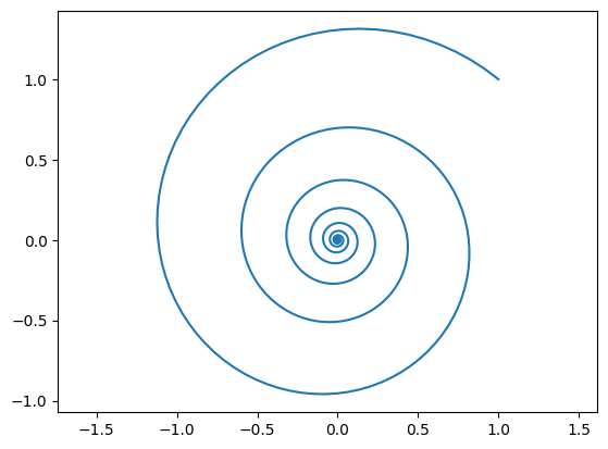
4. Example: Circle / Spiral#
\[\begin{split}
\begin{pmatrix} y \\ x \end{pmatrix} = \begin{pmatrix} \sin{\varphi} \\ \cos{\varphi} \end{pmatrix}
\Leftrightarrow
\begin{pmatrix} \dot{x} \\ \dot{y} \end{pmatrix} = \begin{pmatrix} -y \\ x \end{pmatrix}
\end{split}\]
def F(phi, y):
    myF    = np.zeros(2)
    myF[0] =  -y[1] - 0.1 * y[0]
    myF[1] = y[0] - 0.1 * y[1]
    return myF

N      = 2000
phiMin = 0.01
phiMax = 48.0 * np.pi
phi    = np.linspace(phiMin, phiMax, N)

y0 = [1, 1]     # initial values

sol = integrate.solve_ivp(F, (phiMin, phiMax), y0, t_eval=phi)

plt.figure(1)
plt.plot(sol.y[0,:], sol.y[1,:])
plt.axis('equal')
plt.show()
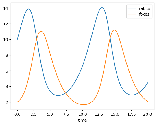
5. Example: Lotka–Volterra equations / predator–prey equations#
\[\begin{split}
\begin{pmatrix} \dot{r} \\ \dot{f} \end{pmatrix} =
\begin{pmatrix} \alpha r - \beta r f \\ \delta r f - \gamma f\end{pmatrix}
\begin{matrix} \text{rabbits} \\ \text{foxes} \end{matrix}
\end{split}\]
a = 0.5
b = 0.1
g = 0.7
d = 0.1

N    = 200
tMin = 0
tMax = 20.0
time = np.linspace(tMin, tMax, N)

y0 = [10, 2]     # initial values

def FLVE(t, y):

    r, f = y

    rDot = a * r     - b * r * f
    fDot = d * r * f - g * f

    return rDot, fDot

sol = integrate.solve_ivp(FLVE, (tMin, tMax), y0, t_eval=time)

plt.figure(1)
plt.plot(time, sol.y[0, :], label="rabits")
plt.plot(time, sol.y[1, :], label="foxes")
plt.legend()
plt.xlabel('time')
plt.show()