Introduction#
The Problem#
import numpy as np
import matplotlib.pyplot as plt
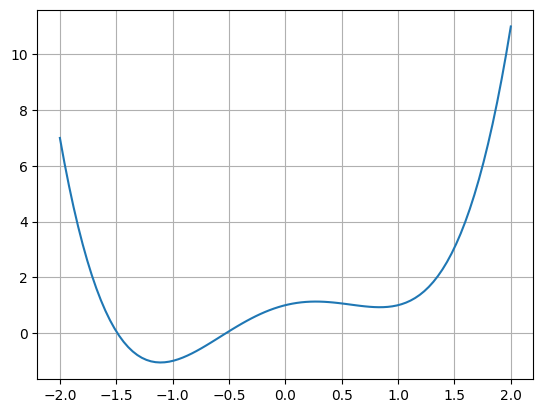
Define and plot our test function:
def f1D(x):
    return x**4.0 - 2.0*x**2.0 + x + 1.0

plt.figure(1)
plt.grid()
x = np.linspace(-2, 2, 100)
plt.plot(x, f1D(x))
plt.show()
The Gradient Descent Algorithm#

def f1D(x):
return x**4.0 - 2.0*x**2.0 + x + 1.0
def df1D(x):
''' defines the derivative of f1D(x)'''
return 4.0*x**3.0 - 4.0*x + 1
plt.figure(1)
plt.grid()
plt.plot(x, f1D(x))
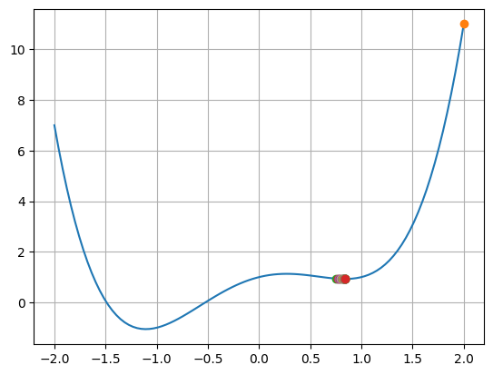
# parameters for the algorithm
x0 = 2.0
gam = 0.05
prec = 0.000001
maxIter = 1000
# gradient descent iteration
for i in range(0, maxIter):
plt.plot(x0, f1D(x0), 'o')
x1 = x0 - gam * df1D(x0)
# check for convergence
if(abs(x0 - x1) <= prec):
break
else:
x0 = x1
print(" Iterations:", i)
print(" x0:", x1)
plt.show()
 Iterations: 42
         x0: 0.8375622023349097
The Conjugate Gradient Algorithm#


See also: https://en.wikipedia.org/wiki/Conjugate_gradient_method
SciPy’s optimize package#
And specifically SciPy’s minimize() function
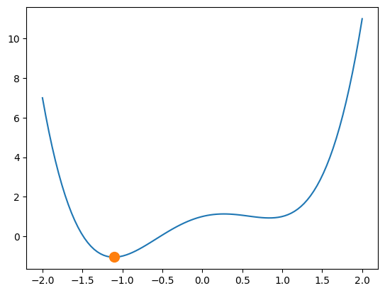
import scipy.optimize as optimize

sol = optimize.minimize(fun=f1D, x0=-2, method='CG')

print( sol )
 message: Optimization terminated successfully.
 success: True
  status: 0
     fun: -1.056172885244464
       x: [-1.107e+00]
     nit: 1
     jac: [ 5.960e-08]
    nfev: 12
    njev: 6
Plot the result:
plt.figure(1)
plt.plot(x, f1D(x))

plt.plot(sol.x, sol.fun, 'o', markersize=10)

plt.show()
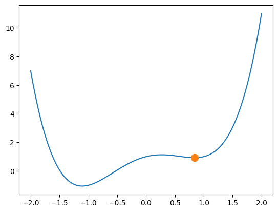
Note
The conjugate gradient method strongly depends on the starting point!
sol = optimize.minimize(fun=f1D, x0=0.5, method='CG')

print( sol )

# and plot it
plt.figure(1)
plt.plot(x, f1D(x))
plt.plot(sol.x, sol.fun, 'o', markersize=10)
plt.show()
 message: Optimization terminated successfully.
 success: True
  status: 0
     fun: 0.9266582180811516
       x: [ 8.376e-01]
     nit: 2
     jac: [-8.941e-08]
    nfev: 12
    njev: 6
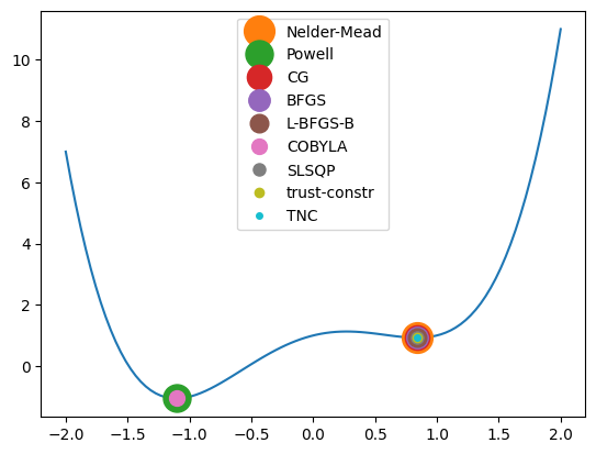
Further methods#
SciPy allows for the following optimization methods:
Nelder-Mead, Powell, CG, BFGS, Newton-CG, L-BFGS-B, TNC, COBYLA, SLSQP, trust-constr, dogleg, trust-ncg, trust-exact, trust-krylov
See
https://docs.scipy.org/doc/scipy/reference/generated/scipy.optimize.minimize.html
https://en.wikipedia.org/wiki/List_of_algorithms#Optimization_algorithms
for details on all of them.
Let’s test those which just need x0:
algorithms = ['Nelder-Mead', 'Powell', 'CG', 'BFGS',
              'L-BFGS-B', 'COBYLA', 'SLSQP', 'trust-constr',
              'TNC']

plt.figure(1)
plt.plot(x, f1D(x))

for i in range(0, len(algorithms)):

    sol = optimize.minimize(fun=f1D, x0=0.5,
                            method=algorithms[i])

    plt.plot(sol.x, sol.fun, 'o', markersize=20-i*2,
             label=algorithms[i])

plt.legend()
plt.show()
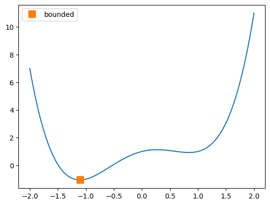
Using bounds instead of \(x_0\)#
plt.figure(1)
plt.plot(x, f1D(x))

sol = optimize.minimize_scalar(fun=f1D, method='bounded',
                               bounds=(-2, 2))

plt.plot(sol.x, sol.fun, 's', markersize=10, label='bounded')

plt.legend()
plt.show()
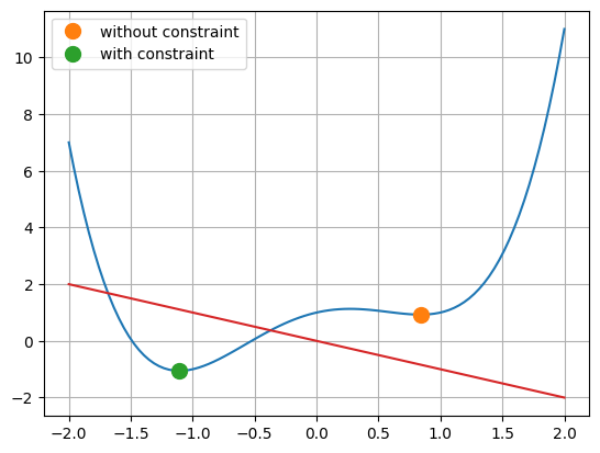
The Full Problem: Including Constraints#
Define an inqeualtity constraint function g1(x) and use it as an inequality constraint using a list of dictonaries:
def g1(x):
    return -x

cons = [{'type': 'ineq',
         'fun' : g1}]

sol     = optimize.minimize(fun=f1D, x0=0.5, method='SLSQP')

solCons = optimize.minimize(fun=f1D, x0=0.5, method='SLSQP',
                            constraints=cons)

plt.figure(1)
plt.grid()
plt.plot(x, f1D(x))

plt.plot(sol.x,     sol.fun,     'o', markersize=10,
         label='without constraint')

plt.plot(solCons.x, solCons.fun, 'o', markersize=10,
         label='with constraint')

plt.plot(x, g1(x))
plt.legend()
plt.show()

print(solCons)
     message: Optimization terminated successfully
     success: True
      status: 0
         fun: -1.056172491482517
           x: [-1.107e+00]
         nit: 5
         jac: [ 2.904e-03]
        nfev: 14
        njev: 5
 multipliers: [ 0.000e+00]
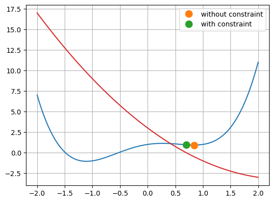
Define an equaltity constraint function h1(x) and use it as an equality constraint using a list of dictonaries:
def h1(x):
    return x**2-5*x+3

cons = [{'type': 'eq',
         'fun' : h1}]

sol = optimize.minimize(fun=f1D, x0=0.5, method='SLSQP')
print( sol )

print("---------")

solCons = optimize.minimize(fun=f1D, x0=0.5, method='SLSQP',
                            constraints=cons)
print( solCons )

# and plot it
plt.figure(1)
plt.grid()
plt.plot(x, f1D(x))

plt.plot(sol.x,     sol.fun,     'o', markersize=10,
         label='without constraint')

plt.plot(solCons.x, solCons.fun, 'o', markersize=10,
         label='with constraint')

plt.plot(x, h1(x))
plt.legend()
plt.show()
     message: Optimization terminated successfully
     success: True
      status: 0
         fun: 0.9266583174268408
           x: [ 8.378e-01]
         nit: 5
         jac: [ 9.373e-04]
        nfev: 11
        njev: 5
 multipliers: []
---------
     message: Optimization terminated successfully
     success: True
      status: 0
         fun: 0.9612951551301436
           x: [ 6.972e-01]
         nit: 4
         jac: [-4.332e-01]
        nfev: 8
        njev: 4
 multipliers: [ 1.201e-01]
The Full Mutli-Dimensional Problem#
a) 2D example 1#
Note
See Matplotlib Plotting for 3D data plotting.
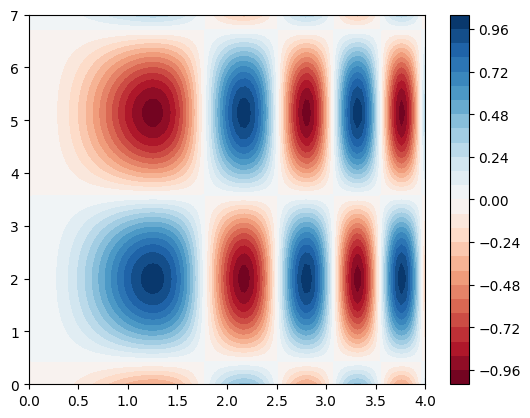
def f2D(x):
    return np.sin(x[0]**2) * np.cos(x[1]-2)

x    = np.linspace(0, 4.0, 100)
y    = np.linspace(0, 7.0, 100)
X, Y = np.meshgrid(x, y)
Z    = f2D([X, Y])

plt.figure(1)
plt.contourf(x, y, Z, cmap='RdBu', levels=30)
plt.colorbar()
plt.show()
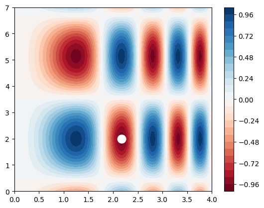
Find “a” minimum in the x/y plane starting from x0 = [2, 3]:
sol = optimize.minimize(fun=f2D, x0=[2, 3])

print( sol )

plt.figure(1)
plt.contourf(x, y, Z, cmap='RdBu', levels=30)

plt.plot(sol.x[0], sol.x[1],
         marker='o', markersize=12, color='w' )

plt.colorbar()
plt.show()
  message: Optimization terminated successfully.
  success: True
   status: 0
      fun: -0.9999999999999997
        x: [ 2.171e+00  2.000e+00]
      nit: 7
      jac: [ 2.980e-08  1.490e-08]
 hess_inv: [[ 5.322e-02  4.948e-04]
            [ 4.948e-04  1.002e+00]]
     nfev: 27
     njev: 9
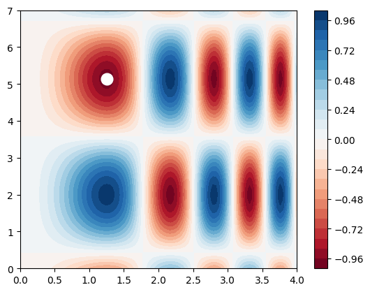
Find “a” minimum in the x/y plane starting from x0 = [2, 5]:
sol = optimize.minimize(fun=f2D, x0=[2, 5])

print( sol )

plt.figure(1)
plt.contourf(x, y, Z, cmap='RdBu', levels=30)

plt.plot(sol.x[0], sol.x[1],
         marker='o', markersize=12, color='w' )

plt.colorbar()
plt.show()
  message: Optimization terminated successfully.
  success: True
   status: 0
      fun: -0.9999999999998982
        x: [ 1.253e+00  5.142e+00]
      nit: 7
      jac: [ 1.177e-06  2.980e-08]
 hess_inv: [[ 1.652e-01  1.122e-03]
            [ 1.122e-03  1.000e+00]]
     nfev: 24
     njev: 8
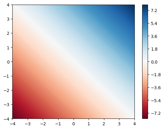
b) 2D example 2#
Hint
Be careful, sometimes the computer is not quite right …
def f2D(x):
    return x[0]+x[1]

sol = optimize.minimize(fun=f2D, x0=[0, 0])

print( sol )

x    = np.linspace(-4, 4.0, 100)
y    = np.linspace(-4, 4.0, 100)
X, Y = np.meshgrid(x, y)
Z    = f2D([X, Y])

plt.figure(1)
plt.contourf(x, y, Z, levels=100, cmap='RdBu')
plt.colorbar()
plt.show()
  message: Optimization terminated successfully.
  success: True
   status: 0
      fun: -258170828.6299674
        x: [-1.291e+08 -1.291e+08]
      nit: 2
      jac: [ 0.000e+00  0.000e+00]
 hess_inv: [[ 5.348e+08  5.348e+08]
            [ 5.348e+08  5.348e+08]]
     nfev: 363
     njev: 121
c) 3D example 1#
def f3D(x):
    return np.sin(x[0]**2 - x[1]) * np.cos(x[2])

sol = optimize.minimize(fun=f3D, x0=[0, 0, 0])

print( sol )
  message: Optimization terminated successfully.
  success: True
   status: 0
      fun: -1.0
        x: [-7.043e-09  1.571e+00 -7.858e-09]
      nit: 4
      jac: [ 0.000e+00  0.000e+00  0.000e+00]
 hess_inv: [[ 1.000e+00  7.139e-10  4.550e-16]
            [ 7.139e-10  1.000e+00 -7.139e-10]
            [ 4.550e-16 -7.139e-10  1.000e+00]]
     nfev: 24
     njev: 6
Note
Remember: more than one (local) minum might exist.
sol = optimize.minimize(fun=f3D, x0=[5, 5, 5])

print( sol )
  message: Optimization terminated successfully.
  success: True
   status: 0
      fun: -0.9999999999998955
        x: [ 4.718e+00  4.983e+00  6.283e+00]
      nit: 9
      jac: [ 3.465e-06 -2.831e-07 -3.353e-07]
 hess_inv: [[ 2.238e-02  1.034e-01 -6.687e-03]
            [ 1.034e-01  9.901e-01 -3.410e-02]
            [-6.687e-03 -3.410e-02  1.028e+00]]
     nfev: 60
     njev: 15
d) 3D example 2: With Constraints#
def f3D(x):
    return np.sin(x[0]**2 - x[1]) * np.cos(x[2])

# and a inequaltiy constraint
# ... i.e. g1(x) >= 0
def g1(x):
    return 1 - x[0]**2 - x[1]**2 - x[2]**2

cons = [{'type': 'ineq',
         'fun': g1}]

sol = optimize.minimize(fun=f3D, x0=[0, 0,0],
                        method='SLSQP', constraints=cons)

print( sol )
print('---------')
print( '   g1(x):', g1(sol.x) )
     message: Optimization terminated successfully
     success: True
      status: 0
         fun: -0.8414709848078964
           x: [-1.490e-08  1.000e+00  0.000e+00]
         nit: 2
         jac: [-7.451e-09 -5.403e-01  7.451e-09]
        nfev: 8
        njev: 2
 multipliers: [ 2.702e-01]
---------
   g1(x): -2.220446049250313e-16