Finding an Optimal Trajectory: The Sliding Particle#

consider a particle that
starts at \(\vec{r}(t=0) = [0,a]\) with \(v(t=0) = v_0\)
slides towards \(\vec{r}(t=T) = [1,b]\)
following the path given by \(\vec{p}(x) = [x, f(x)]\) with \(x \in [0,1]\)
assume \(mg=1\):
\(\Rightarrow\) at position \([x,f(x)]\), its speed \(v(x)\) satisfies: \(\frac12 v(x)^2 = \frac12 v_0^2 + [a-f(x)]\) (initial kinetic + potential energy)
\(\Rightarrow v(x) = \sqrt{v_0^2 + 2[a-f(x)]}\)
direction of \(\vec{v}\) will follow the path given by \(\vec{r}(x) = [x, f(x)]\), i.e. \(\vec{v} \propto \frac{\partial \vec{r}(x)}{\partial x} = [1, f'(x)]\)
\(\Rightarrow\) normalized horizontal speed \(v_h(x) = \frac{v(x)}{\sqrt{1+f'(x)^2}} = \frac{\sqrt{v_0^2 + 2[a-f(x)]}}{\sqrt{1+f'(x)^2}}.\)
Find \(f(x)\) for a given \(v_0\) so that \(T\) is minimized.
Algorithm#

divide interval \(x \in [0,1]\) into \(n\) subintervals: \(x_i= i/n\), for \(i=0,\ldots, n\)
assume that \(f(x)\) is linear on each interval \([x_i, x_{i+1}]\), and continuous on the entire interval \([0,1]\)
\(\Rightarrow\) \(f(x)\) is determined by its value on the points \(x_i\): \(f_i = f(x_i)\)
\(\Rightarrow\) optimize \(T\) over all such functions
Note 1: \(f_0=a\) and \(f_n=b\), since we start at \((0,a)\) and end up at \((1,b)\)
Note 2: \(f\) has a constant derivative on the interval \((x_i, x_{i+1})\): \(f(x)|_{x\in (x_i, x_{i+1})} \approx f_i + f'_i \, (x - x_i)\) $\( \Rightarrow T = \sum_{i=0}^{n-1} \sqrt{1+{f_i'}^2} \int_{x_i}^{x_{i+1}} \frac{dx}{\sqrt{v_0^2 + 2a-2f_i-2f_i'(x-x_i)}}\)$
the integral can now be calculated exactly yielding the functional: $\( \Rightarrow T[f'] = -\sum_{i=0}^{n-1} \frac{\sqrt{1+{f'_i}^2}}{f'_i}\, \left( \sqrt{v_0^2 + 2(a-f_{i+1})} - \sqrt{v_0^2 + 2(a-f_i)}\right)\)$
\(\Rightarrow\) minimize this functional to get optimal \(f'_i\)
\(\Rightarrow\) from this we can easily re-construct \(f_i = a + \sum_{j\le i}f'_j x_j\)
Be careful: For \(v_0=0\), the exact solution \(f\) to the problem is given by a cycloid, which has an infinite derivative at \(x=0\). This leads to large inaccuracies when trying to interpolate the integral.
import numpy as np
import matplotlib.pyplot as plt
import scipy.optimize as optimize
# settings
n = 75
a = 0.4 # starting height
b = 0.0 # ending height
v0 = 0.0 # starting velocity, in the direction of
# the trajectory
dx = 1.0/(n-1)
def Tf(df, v0):
v2 = v0**2
T = 0
for i in range(0, len(df)):
v2new = v2 - 2*df[i]*dx
# in case we found a negative (unphysical)
# new velocity squared we return a huge cost
# such that the algorithm avoids this "solution"
if(v2new < 0):
return 10**10
if(df[i] >= 10**(-9)):
T += np.sqrt( 1 + df[i]**2 ) / df[i] \
* ( np.sqrt(v2) - np.sqrt(v2new) )
else:
# be careful with very small df[i]
T += np.sqrt( 1 + df[i]** 2) \
/ ( np.sqrt(v2) + np.sqrt(v2new) ) \
* 2.0 * dx
# save new v^2 as old one
v2 = v2new
return T
# define equality constraint, so that only solutions
# are chosen which end up at (1, b)
def h1(df):
return sum(df)*dx-(b-a)
cons = ({'type':'eq',
'fun': h1})
# optimize it
sol = optimize.minimize(Tf, x0=[b-a]*(n-1), method='SLSQP',
constraints=cons, args=v0)
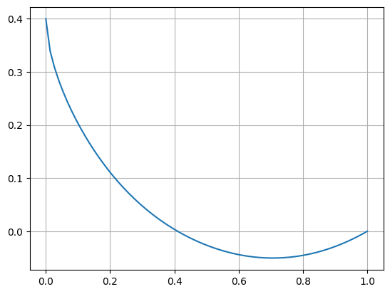
print( Tf(sol.x, v0) )
# plot it
plt.figure(1)
plt.grid()
x = np.linspace(0, 1, n)
plt.plot(x,a+dx*np.cumsum(np.insert(sol.x,0,0)))
plt.show()
1.8136795180800998
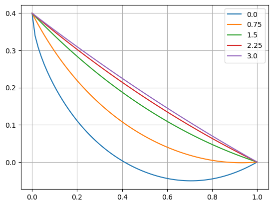
Plot it for varying initial velocities:
plt.figure(1)
plt.grid()

for v0 in np.linspace(0, 3, 5):

    sol = optimize.minimize(Tf, x0=[b-a]*(n-1), method='SLSQP',
                            constraints=cons, args=v0)

    plt.plot(x, a+dx*np.cumsum(np.insert(sol.x,0,0)), label=v0)

plt.legend()
plt.show()
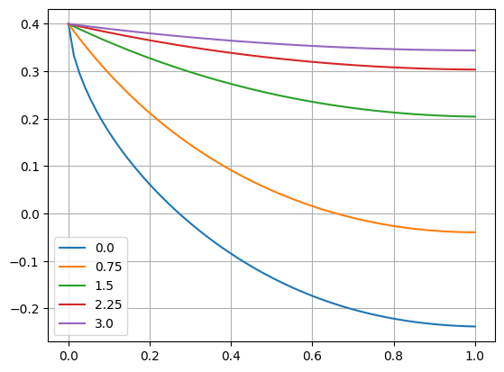
What happens when we remove the constraint?
plt.figure(1)
plt.grid()

for v0 in np.linspace(0, 3, 5):

    sol = optimize.minimize(Tf, x0=[b-a]*(n-1), method='SLSQP',
                            args=v0)

    plt.plot(x, a+dx*np.cumsum(np.insert(sol.x,0,0)), label=v0)

plt.legend()
plt.show()
%%html
<blockquote class="twitter-tweet"><p lang="en" dir="ltr">I built a BRACHISTOCHRONE with <a href="https://twitter.com/tweetsauce?ref_src=twsrc%5Etfw">@tweetsauce</a>! Video: <a href="https://t.co/rC5oktUATG">https://t.co/rC5oktUATG</a> <a href="https://twitter.com/braincandylive?ref_src=twsrc%5Etfw">@braincandylive</a> <a href="https://t.co/sj1FVgqf5v">pic.twitter.com/sj1FVgqf5v</a></p>— Adam Savage (@donttrythis) <a href="https://twitter.com/donttrythis/status/823257178727321600?ref_src=twsrc%5Etfw">January 22, 2017</a></blockquote> <script async src="https://platform.twitter.com/widgets.js" charset="utf-8"></script>
I built a BRACHISTOCHRONE with @tweetsauce! Video: https://t.co/rC5oktUATG @braincandylive pic.twitter.com/sj1FVgqf5v
— Adam Savage (@donttrythis) January 22, 2017
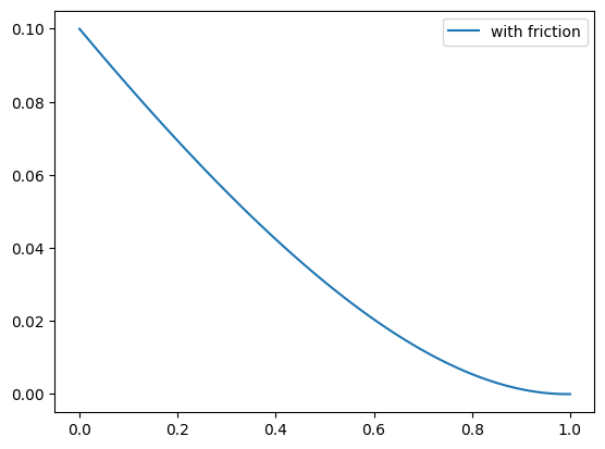
With Friction#
friction: force opposite to the speed of the particle, with magnitude \(\gamma \cdot v\)
differentiated energy equation (measures the change in kinetic energy) becomes
# settings
n = 75
a = 0.1 # starting height
b = 0.0 # ending height (should be < a + 0.5*v^2, because g=1)
dx = 1.0/(n-1)
v0 = 1.5 # 0.9 # starting velocity, in the direction of the trajectory
g = 0.5 # 1.5 # friction constant
def TfFriction(df, v0, g):
v2 = v0**2
T = 0
for i in range(0,len(df)):
# Euler step
v2new = v2 - 2*df[i]*dx - 2*g*np.sqrt(v2)*np.sqrt(1+df[i]**2)*dx
# in case we found a negative new velocity squared
if(v2new < 0):
return 10**10
# T calculation
if(df[i] >= 10**(-9)):
T += np.sqrt( 1 + df[i]**2 ) / df[i] * ( np.sqrt(v2) - np.sqrt(v2new) )
else: # be careful with very small df[i]
T += np.sqrt( 1 + df[i]** 2) / ( np.sqrt(v2) + np.sqrt(v2new) ) * 2.0 * dx
# save new v^2 as old one
v2 = v2new
return T
# define equality constraint, so that only solutions
# are chosen which end up at (1, b)
def h1(df):
return sum(df)*dx-(b-a)
cons=({'type':'eq', 'fun': h1})
# get optimized solution with and without friction
solFriction = optimize.minimize(TfFriction, x0=[b-a]*(n-1), method='SLSQP', constraints=cons, args=(v0, g))
# plot it
plt.figure(1)
x = np.linspace(0, 1, n)
plt.plot(x,a+dx*np.cumsum(np.insert(solFriction.x, 0, 0)), label='with friction')
plt.legend()
plt.show()
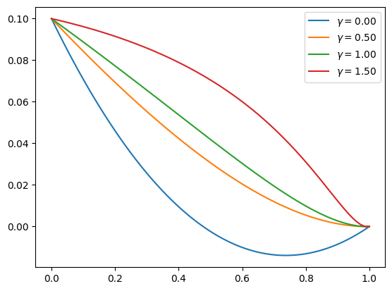
# ... linear parts are prefered
plt.figure(1)

# vary gamma
for g in np.linspace(0, 1.5, 4):
    solFriction = optimize.minimize(TfFriction, x0=[b-a]*(n-1), method='SLSQP', constraints=cons, args=(v0, g))
    plt.plot(x, a+dx*np.cumsum(np.insert(solFriction.x, 0, 0)), label="$\gamma = %3.2f$"%g)

plt.legend()
plt.show()
<>:6: SyntaxWarning: "\g" is an invalid escape sequence. Such sequences will not work in the future. Did you mean "\\g"? A raw string is also an option.
<>:6: SyntaxWarning: "\g" is an invalid escape sequence. Such sequences will not work in the future. Did you mean "\\g"? A raw string is also an option.
/tmp/ipykernel_597/2299117506.py:6: SyntaxWarning: "\g" is an invalid escape sequence. Such sequences will not work in the future. Did you mean "\\g"? A raw string is also an option.
  plt.plot(x, a+dx*np.cumsum(np.insert(solFriction.x, 0, 0)), label="$\gamma = %3.2f$"%g)