Ordinary Differential Equations: Pendulums#
import numpy as np
import matplotlib.pyplot as plt
import scipy.integrate as integrate
import matplotlib
import matplotlib.animation as animation
# set the animation style to "jshtml" (for the use in Jupyter)
matplotlib.rcParams['animation.html'] = 'jshtml'
Simple Pendulum#

Second-oder ODE for the angle \(\varphi\):
\[\large \frac{\partial^2 \varphi}{\partial t^2} = - \frac{g}{l} \sin{\varphi}\]
Coupled system of first-order ODEs:
\[\begin{split} \large \begin{pmatrix}
\dot{\varphi} \\ \dot{\omega}
\end{pmatrix}
=
\begin{pmatrix} \omega \\ - \frac{g}{l} \sin{\varphi} \end{pmatrix}
\end{split}\]
g = 9.8
l = 10.0
tStep = 0.05
tMin = 0
tMax = 20.0
time = np.arange(tMin, tMax, tStep)
y0 = [45/180*np.pi, 0] # initial values
def FPendulum(t, y):
F = np.zeros(2)
F[0] = y[1]
F[1] = -(g/l) * np.sin(y[0])
return F
sol = integrate.solve_ivp(FPendulum,
(tMin, tMax),
y0, t_eval=time)
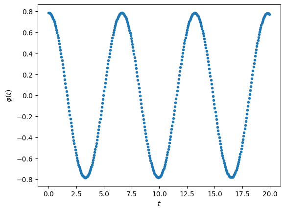
# plot it
plt.figure(1)
plt.plot(sol.t, sol.y[0, :], ".")
plt.xlabel('$t$')
plt.ylabel('$\\varphi(t)$')
plt.show()
Now let’s animate it:
# create figure for the animation
fig = plt.figure(1, figsize = (8,4))
plt.grid()
plt.xlim([-12, 12])
plt.ylim([-11, 1])
# create a mass object for the animation
mass, = plt.plot(0, -l, 'o', markersize=12)
# prevent its showing
plt.close()
# define an animation function
def animate(f):
# get x/y position from phi and l
x = l * np.sin(sol.y[0, f])
y = -l * np.cos(sol.y[0, f])
# move mass to x/y
mass.set_data([x], [y])
# create the animation
frames = np.arange(0, np.size(time))
myAnimation = animation.FuncAnimation(fig,
animate,
frames,
interval=25)
# show animation
myAnimation
# create figure for the animation
fig = plt.figure(1, figsize = (8,4))
plt.grid()
plt.xlim([-12, 12])
plt.ylim([-11, 1])
# create line/mass objects for the animation
line, = plt.plot([0,0], [0, -l])
mass, = plt.plot([0], [-l], 'o', markersize=12)
# prevent its showing
plt.close()
# define an animation function
def animate(i):
# get x/y position from phi and l
x = l * np.sin(sol.y[0, i])
y = -l * np.cos(sol.y[0, i])
# move mass to x/y
mass.set_data([x], [y])
# move line
line.set_data([0, x], [0, y])
# create the animation
frames = np.arange(0, np.size(time))
myAnimation = animation.FuncAnimation(fig,
animate,
frames,
interval=50)
# show animation
myAnimation
Spring Pendulum#

\[\begin{split}\large
\begin{pmatrix} \dot{\theta} \\
\dot{\omega} \\
\dot{r} \\
\dot{v} \\ \end{pmatrix}
=
\begin{pmatrix} \omega \\
-\frac{2}{l+r} v \omega + \omega_\theta^2 sin(\theta) \\
v \\
(l + r) \omega^2 + g cos(\theta) - \omega_r^2 r \\ \end{pmatrix}
\end{split}\]
g = 9.81 # acceleration due to gravity, in m/s^2
M = 1.0 # Mass of attachment in kg
spring = {'m' : 1.0, # Mass of spring in kg
'k' : 100.0, # Spring constant Nm^-1
'l' : 0.1 } # Rest length in m
tStep = 0.05
tMin, tMax = 0, 10.0
time = np.arange(tMin, tMax, tStep)
y0 = np.array([45.0/180.0*np.pi, # initial values
0,
M*g/spring['k'],
0])
def FSpringPendulum(t, y):
'''return derivatives of y = [theta, w, x, v]'''
m = spring['m']
k = spring['k']
l = spring['l']
th, w, x, v = y
wTh = np.sqrt( g / (l + x) )
wR = np.sqrt( k / m )
thDot = w
wDot = -2.0 / (l + x) * v * w - wTh**2.0 * np.sin(th)
xDot = v
vDot = (l + x) * w**2.0 + g * np.cos(th) - wR**2.0 * x
return thDot, wDot, xDot, vDot
sol = integrate.solve_ivp(FSpringPendulum,
(tMin, tMax),
y0, t_eval=time)
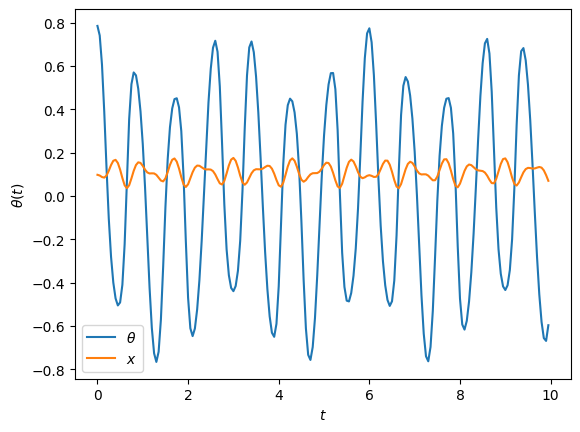
plt.figure(1)
plt.plot(sol.t, sol.y[0, :], label='$\\theta$')
plt.plot(sol.t, sol.y[2, :], label='$x$')
plt.xlabel('$t$')
plt.ylabel('$\\theta(t)$')
plt.legend()
plt.show()
# create figure for the animation
fig = plt.figure(1, figsize = (6,3))
plt.grid()
plt.xlim([-0.505, 0.505])
plt.ylim([-0.5, 0.05])
# create line/mass objects for the animation
line, = plt.plot([0,0], [0, -l])
mass, = plt.plot([0], [-l], 'o', markersize=12)
# prevent its showing
plt.close()
# define an animation function
def animate(i):
# get x/y position from theta, x, and l
l = spring['l']
r = l + sol.y[2, :]
th = sol.y[0, :]
x = r*np.sin(th)
y = -r*np.cos(th)
# move mass to x/y
mass.set_data([x[i]], [y[i]])
# move line
line.set_data([0, x[i]], [0, y[i]])
# create the animation
frames = np.arange(0, np.size(time))
myAnimation = animation.FuncAnimation(fig,
animate,
frames,
interval=75)
# show animation
myAnimation
Double Pendulum#

g = 9.81 # acceleration due to gravity, in m/s^2
L1, L2 = 1.0, 0.51 # length of pendulum 1 and 2 in m
m1, m2 = 4.0, 0.51 # mass of pendulum 1 and 2 in kg
tStep = 0.05
tMin, tMax = 0, 60.0
time = np.arange(tMin, tMax, tStep)
# th10, w10, th20, w20 initial angles and angular velocities
# in degrees / degrees per second
y0 = np.array([170.0, 0.0, 30.0, 0.0]) * np.pi/180.0
def FDoublePendulum(t, y):
'''double pendulum function
with y = [th1, z1, th2, z2]'''
th1, z1, th2, z2 = y
c = np.cos(th1 - th2)
s = np.sin(th1 - th2)
th1dot = z1
z1dot = (m2*g*np.sin(th2)*c - m2*s*(L1*z1**2*c + L2*z2**2) -
(m1+m2)*g*np.sin(th1)) / L1 / (m1 + m2*s**2)
th2dot = z2
z2dot = ((m1+m2)*(L1*z1**2*s - g*np.sin(th2) + g*np.sin(th1)*c) +
m2*L2*z2**2*s*c) / L2 / (m1 + m2*s**2)
return th1dot, z1dot, th2dot, z2dot
sol = integrate.solve_ivp(FDoublePendulum,
(tMin, tMax),
y0, t_eval=time)
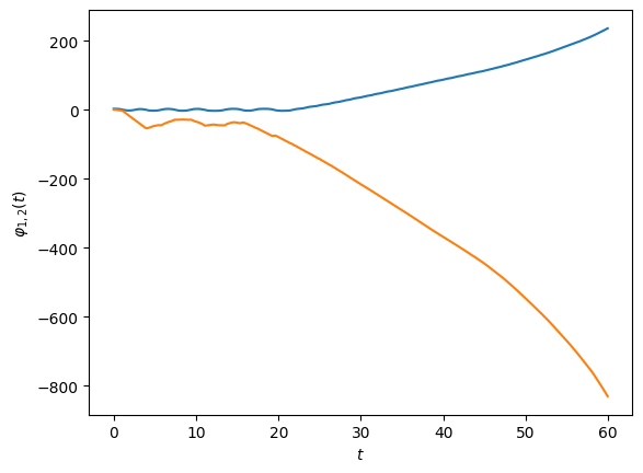
plt.figure(1)
plt.plot(sol.t, sol.y[0, :])
plt.plot(sol.t, sol.y[2, :])
plt.xlabel('$t$')
plt.ylabel('$\\varphi_{1,2}(t)$')
plt.show()
# create figure for the animation
fig = plt.figure(1, figsize = (4,4))
plt.grid()
plt.gca().set_xlim([-1.8, 1.8])
plt.gca().set_ylim([-1.8, 1.8])
# create a line with 2 dots for the animation
line, = plt.plot([0,2,-2], [0,2,-2], 'o-')
# prevent its showing
plt.close()
# define an animation function
def animate(i):
# get x/y position from phi and l for both points
x1 = L1 * np.sin(sol.y[0, i])
y1 = -L1 * np.cos(sol.y[0, i])
x2 = L2 * np.sin(sol.y[2, i]) + x1
y2 = -L2 * np.cos(sol.y[2, i]) + y1
# move line
line.set_data([0, x1, x2], [0, y1, y2])
# create the animation
frames = np.arange(0, np.size(time))
myAnimation = animation.FuncAnimation(fig,
animate,
frames,
interval=25)
# show animation
myAnimation