Numerical Differentiation

---

Warning

This notebook is outdated and should only give you an idea about the topic. Do not use SciPy for numerical differentiation anymore.

# load the standard modules
import matplotlib.pylab as plt
import numpy as np

The Problem & Its Solution

We aim to calculate:

\begin{align*} f’(x) &= \frac{df(x)}{dx} \ &\approx \frac{f(x+d) - f(x)}{d} \ &\approx \frac{f(x+d) - f(x-d)}{2d} \ \text{or} \quad f’’(x) &= \frac{d^2f(x)}{dx^2} \approx \dots \end{align*}

\(\Rightarrow\) Again, we could implement all on our own. Or we could use the predefined functions from Numpy and Numdifftools!

Numerical Differentiation of Analytic Functions

def f(x):
    return np.sin(x)

def fp(x):
    return np.cos(x)

def fpp(x):
    return -np.sin(x)

def fppp(x):
    return -np.cos(x)

# and plot it
x = np.linspace(0, 2.0*np.pi, 100)

plt.figure(1)

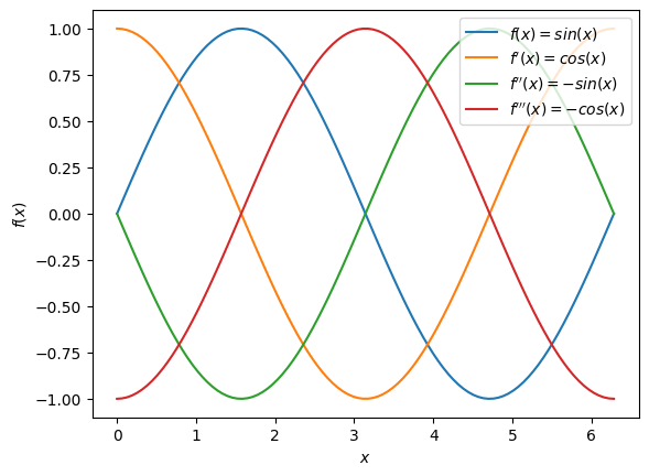
plt.plot(x, f(x),    label="$f(x)    = sin(x)$")
plt.plot(x, fp(x),   label="$f'(x)   = cos(x)$")
plt.plot(x, fpp(x),  label="$f''(x)  = -sin(x)$")
plt.plot(x, fppp(x), label="$f'''(x) = -cos(x)$")

plt.xlabel("$x$")
plt.ylabel("$f(x)$")
plt.legend(loc=1)

plt.show()

import numpy as np
import matplotlib.pyplot as plt
import numdifftools as nd

def f(x):  return np.sin(x)
def fp(x): return np.cos(x)

x0 = 1.23

# n — derivative order
df = nd.Derivative(f, n=1, step=1.5)(x0)
print('df = ', df)

x = np.linspace(0, 2*np.pi, 400)
plt.plot(x, fp(x),     label="$f'(x)=\\cos(x)$")
plt.plot(x0, df, 'ro', label=f"$f'_{{num}}(x={x0:.2f})$")
plt.xlabel("$x$")
plt.ylabel("$f'(x)$")
plt.legend(loc=1)
plt.show()

---------------------------------------------------------------------------
ModuleNotFoundError                       Traceback (most recent call last)
Cell In[3], line 3
      1 import numpy as np
      2 import matplotlib.pyplot as plt
----> 3 import numdifftools as nd
      5 def f(x):  return np.sin(x)
      6 def fp(x): return np.cos(x)

ModuleNotFoundError: No module named 'numdifftools'

x  = np.linspace(0, 2*np.pi, 400)
x0 = 1.23

# Compute numerical derivatives
df   = nd.Derivative(f, n=1, step=0.1)(x0)
ddf  = nd.Derivative(f, n=2, step=0.1)(x0)
dddf = nd.Derivative(f, n=3, step=0.1, order=3)(x0)

# Plot
plt.figure(1)

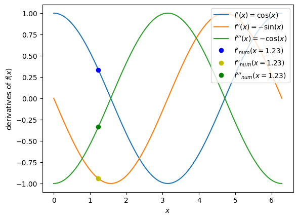
plt.plot(x, fp(x),   label="$f'(x)=\\cos(x)$")
plt.plot(x, fpp(x),  label="$f''(x)=-\\sin(x)$")
plt.plot(x, fppp(x), label="$f'''(x)=-\\cos(x)$")

plt.plot(x0, df,   'bo', label=f"$f'_{{num}}(x={x0:.2f})$")
plt.plot(x0, ddf,  'yo', label=f"$f''_{{num}}(x={x0:.2f})$")
plt.plot(x0, dddf, 'go', label=f"$f'''_{{num}}(x={x0:.2f})$")

plt.xlabel("$x$")
plt.ylabel("derivatives of $f(x)$")
plt.legend(loc=1)
plt.show()

Numerical Differentiation of Sampled Data

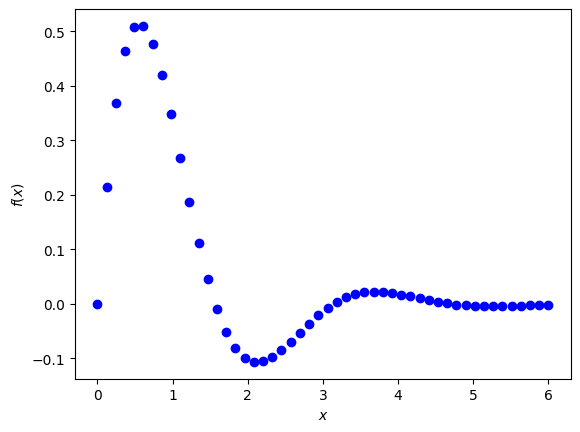
# define some sample data
xi = np.linspace(0, 6, 50)
yi = np.sin(xi/0.5) * np.exp(-xi)

plt.figure(1)
plt.plot(xi, yi, 'bo')

plt.xlabel("$x$")
plt.ylabel("$f(x)$")

plt.show()

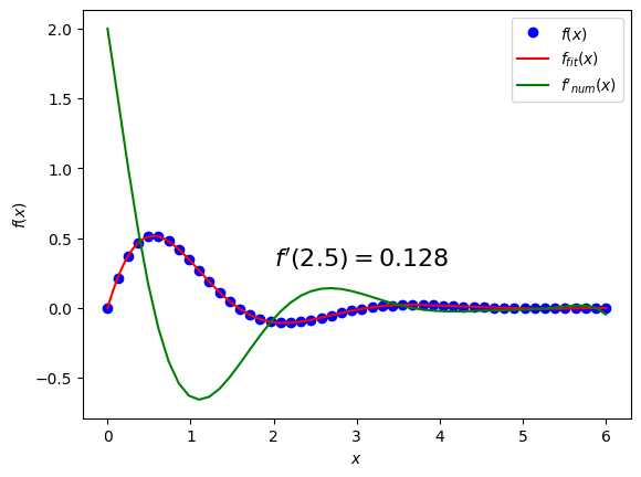
Strategy 1: Fit and use the fit-function in Scipy’s derivative

import numpy as np
import matplotlib.pyplot as plt
import numdifftools as nd

# polynomial approximation
myFit = np.polyfit(xi, yi, deg=9)
fFit = np.poly1d(myFit)

x0 = 2.5

# First derivative
df0 = nd.Derivative(fFit, n=1, step=0.01)(x0)

df = nd.Derivative(fFit, n=1, step=0.01)(xi)

# Plotting
xfine = np.linspace(np.min(xi), np.max(xi), 200)

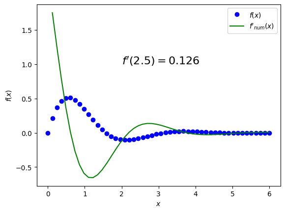
plt.plot(xi, yi, 'bo', label="$f(x)$")
plt.plot(xfine, fFit(xfine), 'r-', label="$f_{fit}(x)$")
plt.plot(xi, df, 'g-', label="$f'_{num}(x)$")
plt.text(2.0, 0.3, f"$f'({x0:.1f}) = {df0:.3f}$", fontsize=16)

plt.xlabel("$x$")
plt.ylabel("$f(x)$")
plt.legend()
plt.show()

Strategy 2: Using Numpy’s diff

# Note: diff returns just f(x_i+1) - f(x_i)
#       so we need to divide by d = x_i - x_i+1 on our own

df = np.diff(yi) / (xi[1] - xi[0])

# find the index of xi which is closest to xx
# (the point at which we'd like to evaluate the differentiation)
ind = np.argmin(np.abs(xi - x0))

plt.text(2.0, 1.0, "$f'(%2.1f) = %4.3f$"%(x0,df[ind]), fontsize=16)

plt.plot(xi, yi, 'bo', label="$f(x)$")
plt.plot(xi[1:], df, 'g-', label="$f'_{num}(x)$") 

plt.xlabel("$x$")
plt.ylabel("$f(x)$")
plt.legend()

plt.show()