Numerical Integration#
The Problem#
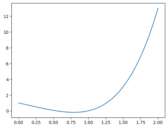
We aim to calculate integrals of the form $\( A = \int_a^b f(x) \, dx\)\( and start with the example: \)\( A = \int_0^2 x^4 - 2x + 1 \, dx\)$ We start with loading modules and with defining and plotting the function:
import matplotlib.pylab as plt
import numpy as np

def f(x):
    return x**4.0 - 2.0 * x + 1.0

plt.figure(1)
x = np.linspace(0, 2, 100)
plt.plot(x, f(x))
plt.show()
Analytic Integration using SymPy#
for a full introduction to SymPy see: https://www.sympy.org
Define our SYMBOLIC variable
import sympy as sp

x = sp.symbols('x')

print( type(x) )
<class 'sympy.core.symbol.Symbol'>
And get the ANALYTIC solution:
A = sp.integrate( f(x), x )

print( A )
-1.0*x**2 + 1.0*x + 0.2*x**5.0
Note
In sp.integrate( f(x), x ) we use a symbol x and the original function f(x)! No need to change this function!
Now let’s evaluate the definite integral.
Variant 1: Via substituting x with 2 and 0:
AAnalytic1 = A.subs(x, 2) - A.subs(x, 0)

print( " variant 1:", AAnalytic1 )
variant 1: 4.40000000000000
Variant 2: Via direct integration:
AAnalytic2 = sp.integrate( f(x), (x, 0, 2) )

print( " variant 2:", AAnalytic2 )
variant 2: 4.40000000000000
Numerical Integration: Rectangle Method / Riemann Sum (midpoint)#

a = 0
b = 2
N = 10

delta = (b - a) / N

xi = np.arange(a + delta / 2.0, b, delta) # excludes b !

print( "step size:", delta )
print( "  xi grid:", xi )
step size: 0.2
  xi grid: [0.1 0.3 0.5 0.7 0.9 1.1 1.3 1.5 1.7 1.9]
Perform the sum via for-loop:
ANum = 0.0
for i in range(0, N):
    ANum += f( xi[i] ) * delta

print( " numerical:", ANum  )
print( "analytical:", AAnalytic1 )
 numerical: 4.346760000000005
analytical: 4.40000000000000
Or more clever using NumPy’s sum():
ANum = np.sum( f( xi ) * delta )

print( " numerical:", ANum  )
print( "analytical:", AAnalytic1 )
 numerical: 4.346760000000005
analytical: 4.40000000000000
Move everything to a function:
def myIntRiemann(f, a, b, N, useNumpy):

    delta = (b - a) / N
    xi = np.arange(a + delta / 2.0, b, delta) # excludes b !

    if(useNumpy == True):
        ANum = np.sum( f(xi) * delta )
    else:
        ANum = 0.0
        for n in range(0, N):
            ANum += f(xi[n]) * delta

    return ANum

print( " numerical:", myIntRiemann(f, a=0, b=2, N=10, useNumpy=False) )
print( "analytical:", AAnalytic1 )
 numerical: 4.346760000000005
analytical: 4.40000000000000
%timeit myIntRiemann(f, a=0, b=2, N=20, useNumpy=False)
%timeit myIntRiemann(f, a=0, b=2, N=20, useNumpy=True)
20.2 μs ± 2.25 μs per loop (mean ± std. dev. of 7 runs, 10,000 loops each)
20.7 μs ± 3.32 μs per loop (mean ± std. dev. of 7 runs, 10,000 loops each)
%timeit myIntRiemann(f, a=0, b=2, N=2000, useNumpy=False)
%timeit myIntRiemann(f, a=0, b=2, N=2000, useNumpy=True)
1.68 ms ± 5.15 μs per loop (mean ± std. dev. of 7 runs, 1,000 loops each)
122 μs ± 3.26 μs per loop (mean ± std. dev. of 7 runs, 10,000 loops each)
print( myIntRiemann(f, a=0, b=2, N=10,  useNumpy=True) )
print( myIntRiemann(f, a=0, b=2, N=20,  useNumpy=True) )
print( myIntRiemann(f, a=0, b=2, N=20000, useNumpy=True) )
print( "analytical:", AAnalytic1 )
4.346760000000005
4.386672500000005
4.399999986666672
analytical: 4.40000000000000
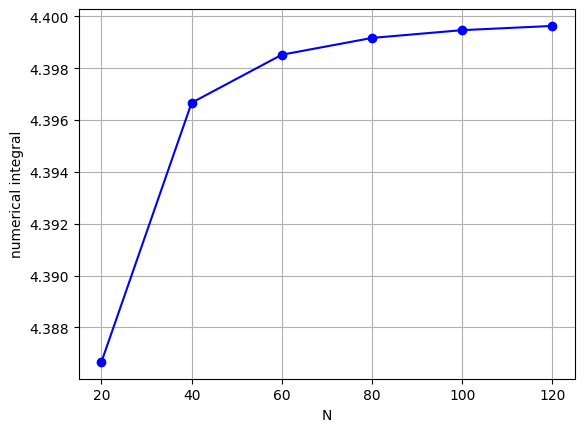
Plot the convergence behaviour:
An = []
nList = np.arange(20, 140, 20)

for n in nList:

    An.append( myIntRiemann(f, a=0, b=2, N=n, useNumpy=True) )

plt.figure(1)
plt.grid(True)

plt.plot(nList, An, 'bo-')

plt.xlabel("N")
plt.ylabel("numerical integral")
plt.show()
Numerical Integration: Trapezoid Method#


see also: https://patrickwalls.github.io/mathematicalpython/integration/trapezoid-rule/
def myIntTrapz(f, a, b, N):

    delta = (b - a) / N
    xi = np.arange(a, b, delta)       # excludes b !!!

    ANum  = f(a) + f(b)
    ANum += 2.0 * np.sum( f(xi[1:]) ) # note: we already excluded b !

    ANum *= delta / 2.0               # don't forget about the step size

    return ANum

print( myIntTrapz(f, a=0, b=2, N=10) )
4.50656
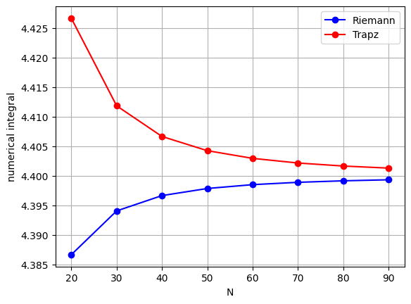
Plot the convergence behaviour:
AnRiemann = []
AnTrapz = []
nList = np.arange(20, 100, 10)

for n in nList:

    AnRiemann.append( myIntRiemann(f, a=0, b=2, N=n, useNumpy=True) )
    AnTrapz.append( myIntTrapz(f, a=0, b=2, N=n) )

plt.figure(1)
plt.grid(True)

plt.plot(nList, AnRiemann, 'bo-', label='Riemann')
plt.plot(nList, AnTrapz, 'ro-', label='Trapz')

plt.xlabel("N")
plt.ylabel("numerical integral")
plt.legend()
plt.show()
Numerical Integration: Gaussian Quadrature#
… similar idea, but more sophisticated weighting functions and automatically chosen steps.
To use it, we need to use SciPy’s integrate sub-module:
import scipy.integrate as integrate
Integrate f from a to b using Gaussian quadrature of order n:
Ann, error = integrate.fixed_quad(f, a=0, b=2, n=3)
print( Ann )
4.400000000000002
Remember that \(f(x) = \frac{1}{5} x^5 - x^2 + x\) is a polynomial function of 5th order. Integration with Gaussian quadrature of order \(n\) is guaranteed to give the exact results for polynomials of order \(2n-1\). Thus \(n=3\) must give the exact result.
Ann, error = integrate.fixed_quad(f, a=0, b=2, n=3)
print( Ann )
4.400000000000002
Integrate f from a to b using Gaussian quadrature of automatic order:
Ann, error = integrate.quad(f, a=0, b=2)
print( Ann )
4.3999999999999995
Compare all methods:
%timeit Ann, error = integrate.quad(f, a=0, b=2)
%timeit Ann        = myIntRiemann(f, a=0, b=2, N=100, useNumpy=True)
%timeit Ann        = myIntTrapz(f, a=0, b=2, N=100)
11.3 μs ± 51.2 ns per loop (mean ± std. dev. of 7 runs, 100,000 loops each)
23.3 μs ± 645 ns per loop (mean ± std. dev. of 7 runs, 10,000 loops each)
25.8 μs ± 5.47 μs per loop (mean ± std. dev. of 7 runs, 10,000 loops each)
Numerical Integration: Comparison#
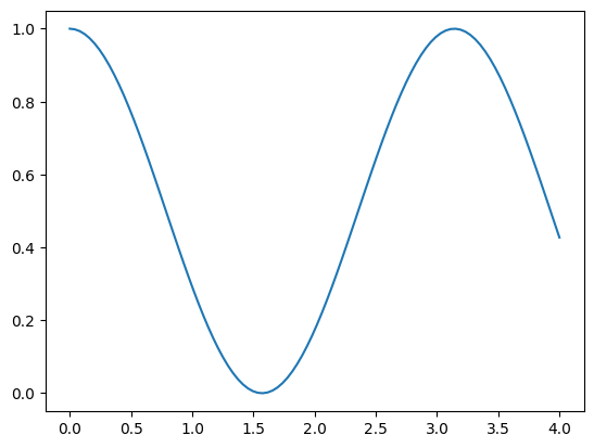
Let’s define another function: $\( A = \int_0^4 cos^2(x) \, dx\)$
def f(x):
    return np.cos(x)**2.0

plt.figure(1)
x = np.linspace(0, 4, 100)
plt.plot(x, f(x))
plt.show()
Plot the convergence behaviour:
AnRiemann = []
AnTrapz = []
AnQuad = []

nList = np.arange(10, 20, 1)

for n in nList:

    AnRiemann.append( myIntRiemann(f, a=0, b=4, N=n, useNumpy=True) )
    AnTrapz.append( myIntTrapz(f, a=0, b=4, N=n) )
    AnQuad.append( integrate.quad(f, a=0, b=4)[0] )

plt.figure(1)
plt.grid(True)

plt.plot(nList, AnRiemann, 'bo-', label='Riemann')
plt.plot(nList, AnTrapz, 'go-', label='Trapz')
plt.plot(nList, AnQuad, 'ro-',  label='Quad')

plt.xlabel("N")
plt.ylabel("numerical integral")
plt.legend()
plt.show()
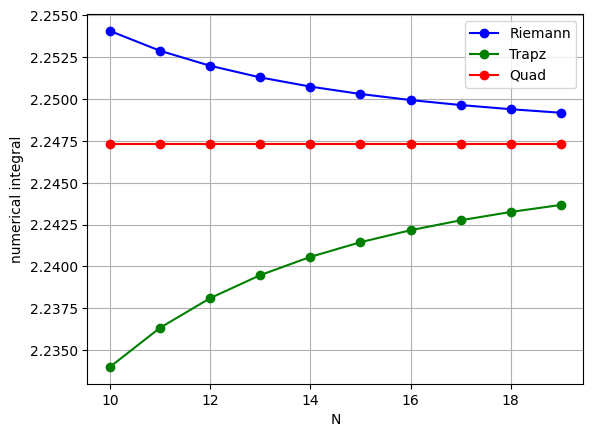
Note
The errors of the Riemann and Trapezoidal depend on the curvature of the function to integrate, the choosen step size, and the integration limits.
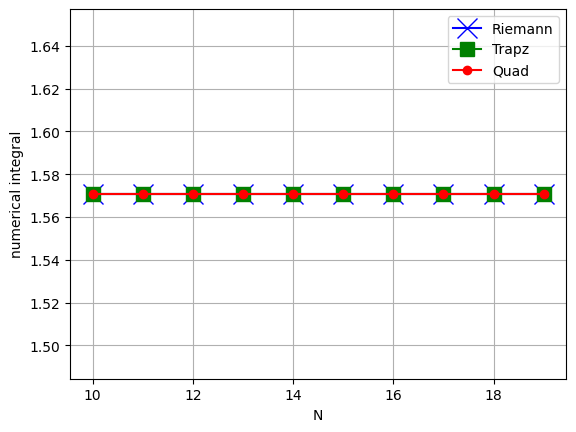
So let’s change the upper limit to \(b=\pi\):
AnRiemann = []
AnTrapz = []
AnQuad = []

nList = np.arange(10, 20, 1)

for n in nList:

    AnRiemann.append( myIntRiemann(f, a=0, b=np.pi, N=n, useNumpy=True) )
    AnTrapz.append( myIntTrapz(f, a=0, b=np.pi, N=n) )
    AnQuad.append( integrate.quad(f, a=0, b=np.pi)[0] )

plt.figure(1)
plt.grid(True)

plt.plot(nList, AnRiemann, 'bx-', label='Riemann', markersize=14)
plt.plot(nList, AnTrapz, 'gs-', label='Trapz', markersize=10)
plt.plot(nList, AnQuad, 'ro-',  label='Quad')

plt.xlabel("N")
plt.ylabel("numerical integral")
plt.legend()
plt.show()
\(\pm \infty\) as Integral Limits#
Use a simple substitution:
\begin{align*} x &= \frac{z}{1-z} \ \Rightarrow dx &= \frac{z , dz}{(1-z)^2} + \frac{dz}{1-z} \ \Rightarrow A &= \int_0^{1} e^{-\frac{z}{1-z}} \left( \frac{z}{(1-z)^2} + \frac{1}{1-z} \right) dz \end{align*} which translates to:
def f(z):
    return np.exp(-z/(1-z)) * (z / (1-z)**2 + 1 / (1-z))

A, error = integrate.quad(f, a=0, b=1)
print( A )
0.9999999999999996
… or just use np.inf as the upper limit!
def f(x):
    return np.exp(-x)

A, error = integrate.quad(f, a=0, b=np.inf)
print( A )
1.0000000000000002
See https://en.wikipedia.org/wiki/Gaussian_quadrature#Other_forms to understand how this works.
Integration of Sampled Data#
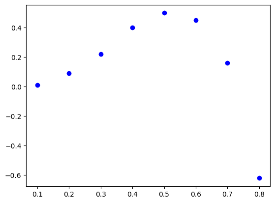
So far we had a well defined function \(y = f(x)\). But what should we do if we have just a sampled data set like \(y_i = f(x_i)\) on a discrete set of \(x_i\) points?
# define some sample data
xi = np.array([0.10, 0.20, 0.30, 0.40, 0.50, 0.60, 0.70,  0.80])
yi = np.array([0.01, 0.09, 0.22, 0.40, 0.50, 0.45, 0.16, -0.62])

plt.figure(1)
plt.plot(xi, yi, 'bo')
plt.show()
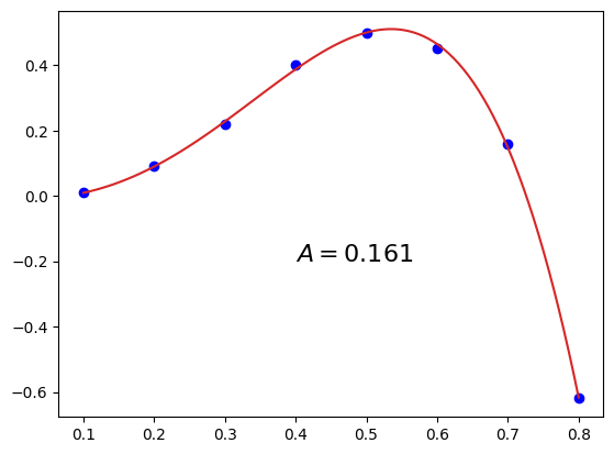
Strategy 1: Fit and use the fit-function in SciPy’s quad():#
We can use, for example, a polynomial function for the fit:
plt.figure(1)
plt.plot(xi, yi, 'bo')

myFit = np.polyfit(xi, yi, deg=4)
f = np.poly1d(myFit)

xfine = np.linspace(np.min(xi), np.max(xi), 100)
plt.plot(xfine, f(xfine), 'tab:red')

# and integrate this one via quad
A, error = integrate.quad(f, a=np.min(xi), b=np.max(xi))
plt.text(0.4, -0.2, "$A = %4.3f$"%A, fontsize=16)

plt.show()
Strategy 2: Use trapezoidal or Simpson’s rule from scipy.integrate:#
Remember that these methods (such as \( A = \int_a^b f(x) \, dx \approx \sum_{i=0}^{N-1} f(x_i) \Delta_i\)) actually only need pairs of \(x_i\) and \(f(x_i)\).
ATrapz = np.trapezoid(yi, x=xi)
print( ATrapz )
0.15149999999999997
import scipy
ASimps = scipy.integrate.simpson(yi, dx=0.1)
print( ASimps )
0.16008333333333333
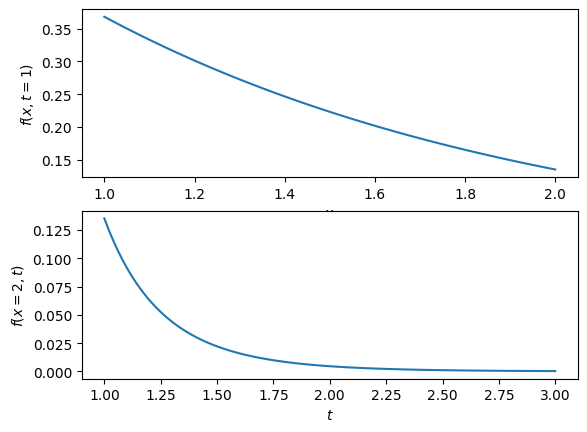
Multi-dimensional Integrals#
def f(x,t):
    return np.exp(-x*t) / t**2.0

x = np.linspace(1, 2, 100)
t = np.linspace(1, 3, 100)

plt.figure(1)

plt.subplot(2, 1, 1)
plt.plot(x, f(x, 1))
plt.xlabel('$x$')
plt.ylabel('$f(x,t=1)$')

plt.subplot(2, 1, 2)
plt.plot(t, f(2, t))
plt.xlabel('$t$')
plt.ylabel('$f(x=2,t)$')

plt.show()
Multi-dimensional integral via SciPy’s integrate.nquad():#
xa = 0
xb = 2

ta = 1
tb = 3

A, error = integrate.nquad(f, [[xa, xb],
                               [ta, tb]])

print( A )
0.4143426872796576
Infinite limits
xa = 0
xb = np.inf

ta = 1
tb = np.inf

A, error = integrate.nquad(f, [[xa, xb],
                               [ta, tb]])

print( A )
0.4999999999999961