Monte Carlo Techniques

---

import numpy as np
import matplotlib.pyplot as plt

# animated
import matplotlib
import matplotlib.animation as animation
# set the animation style to "jshtml" (for the use in Jupyter)
matplotlib.rcParams['animation.html'] = 'jshtml'

Monte Carlo Integration

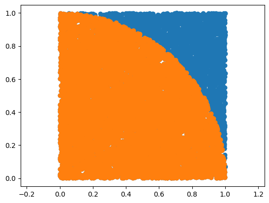
a) Calculating \(\pi\)

\[ r = \sqrt{x^2 + y^2} \]

1. generate \(N\) random \((x,y)\) pairs with \(0 \le x,y \le 1\)

2. calculate \(r\) for all of them

3. count how many pairs (\(n\)) lay inside the circle (\(r \le 1\))

4. from \(A = \pi r^2\) we than get: \(\pi = \frac{4n}{N}\)

N    = 10000
x, y = np.random.rand(2, N)
r    = np.sqrt(x**2.0 + y**2.0)
mypi = 4.0*len( r[r <= 1] ) / N

print("  MC Pi =", mypi)
print("  Error :", 100*(1.0 - mypi/np.pi), "%")

plt.figure(1)
plt.plot(x, y, 'o')
plt.plot(x[r < 1], y[r < 1], 'o')
plt.axis("equal")
plt.show()

  MC Pi = 3.1508
  Error : -0.29307893878876 %

b) Multi-dimensional volume (n-dim sphere)

np.random.seed(123)

def getNDimSphereVol(dim):
    N    = 1000000
    x    = np.random.rand(dim, N)
    dist =  np.sum( x**2, axis=0 )
    vol  = 2.0**dim * len(dist[dist<1]) / N
    return vol

print('   0D: %f  vs.  %f  R^0'%(getNDimSphereVol(dim=0), 1))
print('   1D: %f  vs.  %f  R^1'%(getNDimSphereVol(dim=1), 2))
print('   2D: %f  vs.  %f  R^2'%(getNDimSphereVol(dim=2), 3.142))
print('   3D: %f  vs.  %f  R^3'%(getNDimSphereVol(dim=3), 4.189))
print('   4D: %f  vs.  %f  R^4'%(getNDimSphereVol(dim=4), 4.935))
print('   5D: %f  vs.  %f  R^5'%(getNDimSphereVol(dim=5), 5.264))
print('   6D: %f  vs.  %f  R^6'%(getNDimSphereVol(dim=6), 5.168))
print('   7D: %f  vs.  %f  R^7'%(getNDimSphereVol(dim=7), 4.725))

   0D: 1.000000  vs.  1.000000  R^0
   1D: 2.000000  vs.  2.000000  R^1
   2D: 3.140652  vs.  3.142000  R^2

   3D: 4.185720  vs.  4.189000  R^3
   4D: 4.940704  vs.  4.935000  R^4

   5D: 5.249216  vs.  5.264000  R^5

   6D: 5.180992  vs.  5.168000  R^6
   7D: 4.736000  vs.  4.725000  R^7

1000000**(1./7.)

7.196856730011519

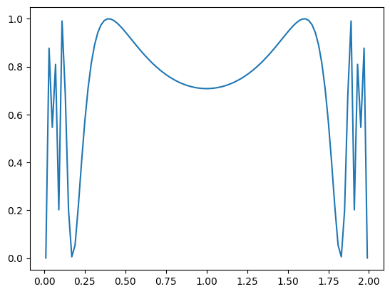
Monte Carlo Mean Values

\[ f(x) = \left[ \sin \left({ \frac{1}{x (2 - x)} } \right) \right]^2\]

def f(x):
    return (np.sin(1/(x*(2-x))))**2

dx = 0.01
x  = np.linspace(dx, 2.0-dx, 100)

print( "Simple mean:", np.mean(f(x)) )

plt.figure(1)
plt.plot(x, f(x))
plt.show()

Simple mean: 0.728999486125733

N = 1000000
x = 2.0 * np.random.rand(N)
y = f(x)
I = 2.0/N * y.sum()

print( "MC mean:", np.mean(f(x)) )

MC mean: 0.7258550606385165

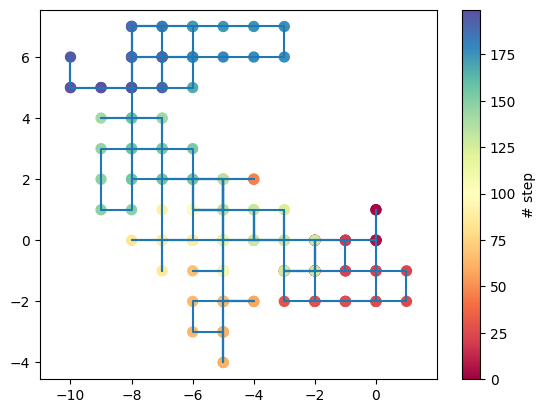
Random Walks

• path that consists of a succession of random steps

• examples include:

  • path traced by a molecule as it travels

  • price of a fluctuating stock

  • financial status of a gambler

  • …

• have applications to ecology, psychology, computer science, physics, chemistry, biology, ..

• closely connected to Markov chains (sequence of possible events in which the probability of each event depends only on the state from the previous event)

https://en.wikipedia.org/wiki/Random_walk / https://en.wikipedia.org/wiki/Markov_chain

def randomWalk(length):
    
    walk = np.zeros((length, 2))
    
    for i in range(1, length):
        
        walk[i, :] = walk[i-1, :]
        
        # toss a 4-side coin to decide where to go
        new = np.random.randint(1,5) # randomly choose from 1,2,3,4
        
        if(new == 1):
            walk[i, 0] += 1
        elif(new == 2):
            walk[i, 1] += 1
        elif(new == 3):
            walk[i, 0] -= 1
        else:
            walk[i, 1] -= 1

    return walk

nStep = 200
walk  = randomWalk(nStep)

plt.figure(1)
plt.plot(walk[:, 0], walk[:, 1], label= 'Random walk')
plt.scatter(walk[:, 0], walk[:, 1], s=51, c=range(nStep), cmap='Spectral')
plt.colorbar(label='# step')
plt.axis('equal')
plt.show()

# animated
import matplotlib
import matplotlib.animation as animation
# set the animation style to "jshtml" (for the use in Jupyter)
matplotlib.rcParams['animation.html'] = 'jshtml'
    
fig = plt.figure()
line,  = plt.plot(walk[:, 0],walk[:, 1], '-')
point, = plt.plot([0,0], [0,0], 'o')
plt.axis('equal')
plt.close()

def init():
    line.set_data([], [])
    return line,

def animate(i):
    x = walk[:i, 0]
    y = walk[:i, 1]
    line.set_data(x, y)
    if (i > 0):
        point.set_data([x[-1]],[y[-1]])
    return line, point

myAnimation = animation.FuncAnimation(fig, animate, init_func=init,
                                      frames=nStep, interval=100, blit=True)
myAnimation

Once Loop Reflect

Random Surfer: PageRank

• \(p_i\): pages under consideration

• \(M(p_i)\): set of pages that link to \(p_{i}\)

• \(N\): total number of pages

• \(d\): probability that a surfer jumps randomly

• \(L\): number of links on page

\(\Rightarrow\) can be iteratively evaluated, calculated as an eigenvalue problem, or using a random surfer

# Website Graph:
#
#     0---1
#     | 4 |
#     3---2

# define nodes and their links
nodes    = dict()
nodes[0] = np.array([1,3,4])    # node / website 0 is connected to 1,3,4
nodes[1] = np.array([0,2,4])    #                1                 0,2,4
nodes[2] = np.array([1,3,4])    # ...
nodes[3] = np.array([0,2,4])
nodes[4] = np.array([0,1,2,3])

def getPageRank(nodes, nSteps):

    nodesCount = np.zeros(len(nodes))
    
    pos = 4 # initial position
    
    for i in range(0, nSteps):

        # toss a coin
        r = np.random.rand()

        # click random link on actual side
        if(r <= 0.85):
            rl  = np.random.randint(len(nodes[pos]))
            pos = nodes[pos][rl]
        # jump to random page
        else:
            pos = np.random.randint(len(nodes))

        nodesCount[pos] += 1

    return nodesCount[:] / np.sum(nodesCount)

PageRank = getPageRank(nodes, 100000)

print("  Node    PageRank")
print("  ----------------")
for i in range(len(nodes)):
    print("    %2d       %4.3f"%(i, PageRank[i]))

  Node    PageRank
  ----------------
     0       0.189
     1       0.188
     2       0.190
     3       0.191
     4       0.242

# Website Graph: ... why it can be (could have been) worth to buy links
#
#     0---1
#     | 4 |
#     3---2--5
#         |
#         6

nodes    = dict()
nodes[0] = np.array([1,3,4])
nodes[1] = np.array([0,2,4])
nodes[2] = np.array([1,3,4,5,6])
nodes[3] = np.array([0,2,4])
nodes[4] = np.array([0,1,2,3])
nodes[5] = np.array([2])
nodes[6] = np.array([2])

PageRank = getPageRank(nodes, 100000)

print("  Node    PageRank")
print("  ----------------")
for i in range(len(nodes)):
    print("    %2d       %4.3f"%(i, PageRank[i]))

  Node    PageRank
  ----------------
     0       0.143
     1       0.145
     2       0.252
     3       0.144
     4       0.187
     5       0.065
     6       0.064

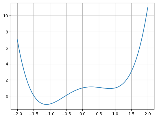
Metropolis Algorithm / Simulated Annealing

a) Minimization via Metropolis

# define our function
def f1D(x):
    return x**4.0 - 2.0*x**2.0 + x + 1.0

# and plot it
plt.figure(1)
plt.grid()
x = np.linspace(-2, 2, 100)
plt.plot(x, f1D(x))
plt.show()

# Metropolis algorithm
def getMinimumMet(f, N, kT):
    
    moves = np.zeros(N)
    
    x0 = 1.5 # initial position
    for i in range(0, N):

        # save the move
        moves[i] = x0

        # get random number between -2 and +2
        step = np.random.rand() * 1.0 - 0.5
        x1 = x0 + step

        if x1 > 2:
            x1 = 2

        if x1 <-2:
            x1 = -2
        
        #x1 = np.random.rand() * 4.0 - 2.0

        # if new x results in smaller f(x) we accept the move immediately
        if(f(x1) <= f(x0)):
            x0 = x1
        else:
            # otherwise we toss a coin
            r = np.random.rand()
            # and define acceptance (Boltzmann probability)
            P = np.exp(- (f(x1) - f(x0)) / kT)
            if(r < P):
                x0 = x1
                
    return moves

moves = getMinimumMet(f=f1D, N=400, kT=1.0)
    
# plot and animate the steps
fig = plt.figure()
x = np.linspace(-2, 2, 100)
plt.plot(x, f1D(x))
point,  = plt.plot([0,0], [0,0], 'o')
point2, = plt.plot([0,0], [0,0], 'o', markersize=12)
plt.close()

def animate(i):
    point.set_data(moves[0:i], f1D(moves[0:i]))
    point2.set_data([moves[i]], [f1D(moves[i])])

myAnimation = animation.FuncAnimation(fig, animate, frames=len(moves), interval=20)
myAnimation

Once Loop Reflect

#moves = getMinimumMet(f=f1D, N=50,   kT=10.0)
#moves = getMinimumMet(f=f1D, N=400,  kT=10.0)
#moves = getMinimumMet(f=f1D, N=400,  kT=1.0)
moves = getMinimumMet(f=f1D, N=400,  kT=0.01)
    
fig = plt.figure()
x = np.linspace(-2, 2, 100)
plt.plot(x, f1D(x))
plt.plot(moves, f1D(moves), 'o')
plt.plot(moves[-1], f1D(moves[-1]), 'o', markersize=12)
plt.show()

b) 1D Optimization via Simulated Annealing

def getMinimumSA(f, N, kT0, kT1):
    
    # define a "cooling" schedule
    kT    = np.linspace(kT0, kT1, N)
    
    moves = np.zeros(N)
    x0    = 2.0
    for i in range(0, N):

        # save the move
        moves[i] = x0

        # get random number between -2 and +2
        # x1 = np.random.rand() * 4.0 - 2.0

        step = np.random.rand() * 1.0 - 0.5
        x1 = x0 + step

        if x1 > 2:
            x1 = 2

        if x1 <-2:
            x1 = -2
        
        # if new x results in smaller f(x) we accept the move immediately
        if(f(x1) <= f(x0)):
            x0 = x1
        else:
            # otherwise we toss a coin
            r = np.random.rand()
            # and define acceptance (Boltzmann probability)
            P = np.exp(- (f(x1) - f(x0)) / kT[i])
            if(r < P):
                x0 = x1
                
    return moves

moves = getMinimumSA(f=f1D, N=450, kT0=10.0, kT1=0.001)
    
fig = plt.figure()
x = np.linspace(-2, 2, 1000)
plt.plot(x, f1D(x))
plt.plot(moves, f1D(moves), 'o')
plt.plot(moves[-1], f1D(moves[-1]), 'o', markersize=12)
plt.show()

# define a function with several local minima
def f1DSin(x):
    return x**4.0 - 2.0*x**2.0 + x + 1.0 + np.sin(x*12.0) + np.sin(x*17.0)

# and plot it
plt.figure(1)
plt.grid()
x = np.linspace(-2, 2, 500)
plt.plot(x, f1DSin(x))
plt.show()

moves = getMinimumSA(f=f1DSin, N=1000, kT0=5.0, kT1=0.01)
    
fig = plt.figure()
plt.grid(True)
x = np.linspace(-2, 2, 500)
plt.plot(x, f1DSin(x))
plt.plot(moves, f1DSin(moves), 'o')
plt.plot(moves[-1], f1DSin(moves[-1]), 'o', markersize=12)
plt.show()