Fitting via Optimization

---

import numpy as np
import matplotlib.pyplot as plt
import scipy.optimize as optimize

Fitting Simple Functions

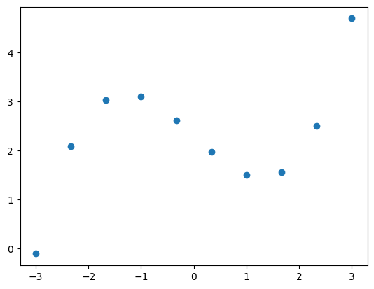
xi = np.linspace(-3, 3, 10)
yi = 0.2 * xi**3.0 - 1.0 * xi + 2.3

plt.figure(1)
plt.plot(xi, yi, 'o')
plt.show()

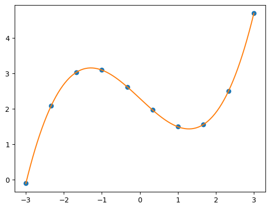
In the following we define fit(x,c) as our generic fitting function. To find the optimal fitting parameters c (a list here), we further define a cost function cost(c), which measures the quality of the fit by calculating $\( cost(\vec{c}) = \sum_i |y_i - f(x_i, \vec{c} )|^2, \)\( where \)y_i\( is the original data and \)f(x_i, \vec{c})$ our fit. Afterwards we use optimize.minimize() to minimize the cost function via finiding the optimal parameters c. With the chosen cost function, this equivalent to a least-square fit.

def fit(x, c):
    return c[0] * x**3.0 + c[1] * x + c[2]
    
    #return c[0] * np.cos(x - c[1]) + c[2] * x + c[3]

def cost(c):
    return np.sum( np.abs( yi - fit(xi, c) )**2.0 )

sol = optimize.minimize(fun=cost, x0=[0, 0, 0, 0], 
                        method='SLSQP')

print(sol)

     message: Optimization terminated successfully
     success: True
      status: 0
         fun: 5.181077947482736e-13
           x: [ 2.000e-01 -1.000e+00  2.300e+00  0.000e+00]
         nit: 5
         jac: [ 5.241e-09  8.601e-10  1.932e-11  0.000e+00]
        nfev: 32
        njev: 5
 multipliers: []

xPlot = np.linspace(-3, 3, 100)
plt.figure(1)
plt.plot(xi, yi, 'o')

plt.plot(xPlot, fit(xPlot, sol.x))

plt.show()

Fitting Noisy Data

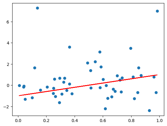
n = 50
x = np.random.rand(n)

# heavly tailed random errors
y_clean = 2.0*x - 1.0
y = 2.0*x - 1.0 + np.random.standard_t(df=2, size=n) 

plt.figure(1)
plt.plot(x, y, 'o')
plt.plot(x, y_clean, 'r-')
plt.show()

def fit(x, c):
    return c[0] * x + c[1]

# least-square cost function
def costL2(c, xi, yi):
    return np.sum( np.abs( yi - fit(xi, c) )**2.0 )

# absolute error cost function
def costL1(c, xi, yi):
    return np.sum( np.abs( (yi - fit(xi, c)) ) )

n     = 50
N     = 1000
errL2 = np.zeros(N)
errL1 = np.zeros(N)

for i in range(N):

    x = np.random.rand(n)
    y = 2.0*x - 1.0 + np.random.standard_t(df=2, size=n)
    
    solL2    = optimize.minimize(fun=costL2, x0=[0, 0], 
                                 method='SLSQP', args=(x, y))
    errL2[i] = np.abs(solL2.x[0] - 2)
    
    solL1    = optimize.minimize(fun=costL1, x0=[0, 0], 
                                 method='SLSQP', args=(x, y))
    errL1[i] = np.abs(solL1.x[0] - 2)

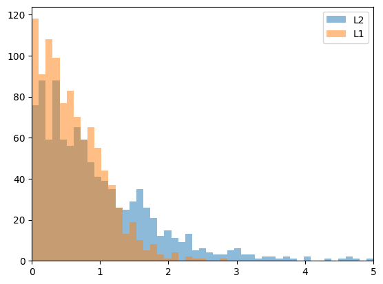
print(" L2 mean:", np.mean(errL2))
print(" L1 mean:", np.mean(errL1))
    
plt.figure(1)
plt.hist(errL2, bins=np.linspace(0,5,50), 
         label='L2', alpha=0.5)
plt.hist(errL1, bins=np.linspace(0,5,50), 
         label='L1', alpha=0.5)
plt.xlim([0, 5])
plt.legend()
plt.show()

 L2 mean: 1.0278534128251526
 L1 mean: 0.6015541731084001

def fit(x, c):
    return c[0] * x + c[1]

# least-square cost function
def costL2(c, xi, yi):
    return np.sum( np.abs( yi - fit(xi, c) )**2.0 )

# absolute error cost funciton
def costL1(c, xi, yi):
    return np.sum( np.sqrt( (yi - fit(xi, c))**2.0 ) )

# logarithmic error cost function
def costLLog(c, xi, yi):
    return np.sum(np.log(( fit(xi, c) - yi)**2.0 + 1.0))

n     = 50
N     = 1000
errL2 = np.zeros(N)
errL1 = np.zeros(N)
errLLog = np.zeros(N)

for i in range(N):

    x = np.random.rand(n)
    y = 2.0*x - 1.0 + np.random.standard_t(df=2, size=n) 
    
    solL2      = optimize.minimize(fun=costL2, x0=[0, 0], 
                                   method='SLSQP', args=(x, y))
    errL2[i]   = np.abs(solL2.x[0] - 2.0)
    
    solL1      = optimize.minimize(fun=costL1, x0=[0, 0], 
                                   method='SLSQP', args=(x, y))
    errL1[i]   = np.abs(solL1.x[0] - 2.0)
    
    solLLog    = optimize.minimize(fun=costLLog, x0=[0, 0], 
                                   method='SLSQP', args=(x, y))
    errLLog[i] = np.sqrt((solLLog.x[0] - 2)**2)

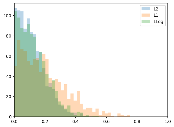
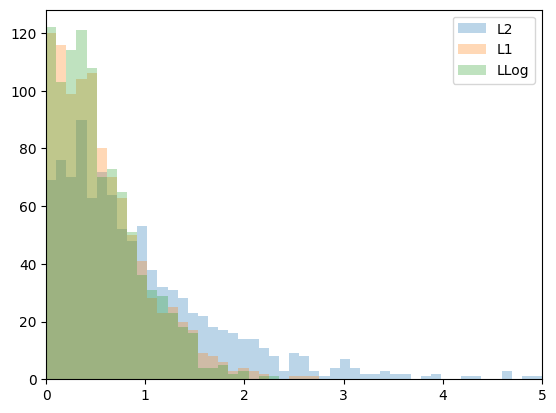
print("   L2 mean:", np.mean(errL2))
print("   L1 mean:", np.mean(errL1))
print(" LLog mean:", np.mean(errLLog))
    
plt.figure(1)
plt.hist(errL2,   bins=np.linspace(0,5,50), 
         label='L2',   alpha=0.3)
plt.hist(errL1,   bins=np.linspace(0,5,50), 
         label='L1',   alpha=0.3)
plt.hist(errLLog, bins=np.linspace(0,5,50), 
         label='LLog', alpha=0.3)
plt.xlim([0, 5])
plt.legend()
plt.show()

   L2 mean: 0.9933721689676688
   L1 mean: 0.5684948908980173
 LLog mean: 0.5416548165228569

# using white noise error
errL2 = np.zeros(N)
errL1 = np.zeros(N)
errLLog = np.zeros(N)

for i in range(N):

    x = np.random.rand(n)
    y = 2.0*x - 1.0 + np.random.rand(n) # white noise error
    
    solL2      = optimize.minimize(fun=costL2, x0=[0, 0], 
                                   method='SLSQP', args=(x, y))
    errL2[i]   = np.abs(solL2.x[0] - 2.0)
    
    solL1      = optimize.minimize(fun=costL1, x0=[0, 0], 
                                   method='SLSQP', args=(x, y))
    errL1[i]   = np.abs(solL1.x[0] - 2.0)
    
    solLLog    = optimize.minimize(fun=costLLog, x0=[0, 0], 
                                   method='SLSQP', args=(x, y))
    errLLog[i] = np.sqrt(np.sum((solLLog.x[0] - 2)**2))

print("   L2 mean:", np.mean(errL2))
print("   L1 mean:", np.mean(errL1))
print(" LLog mean:", np.mean(errLLog))
    
plt.figure(1)
plt.hist(errL2,   bins=np.linspace(0,1,50), 
         label='L2',   alpha=0.3)
plt.hist(errL1,   bins=np.linspace(0,1,50), 
         label='L1',   alpha=0.3)
plt.hist(errLLog, bins=np.linspace(0,1,50), 
         label='LLog', alpha=0.3)
plt.xlim([0, 1])
plt.legend()
plt.show()

   L2 mean: 0.11838018024314924
   L1 mean: 0.19834605402651811
 LLog mean: 0.12783320665351436