(Discrete) Fourier Transforms#
Introduction#
For continuous functions (e.g.):
\[ \large \begin{align} \hat{f}(y) = \int f(x) \, e^{-iy\cdot x} \, dx \quad \Leftrightarrow \quad f(x) = \frac{1}{(2\pi)^n} \int \hat{f}(y) \, e^{iy\cdot x} \, dy \end{align} \]For sampled data we need to use the discrete Fourier transform (DFT):
\[ \large \begin{align} y_k = \sum_{n=0}^{N-1} e^{-2\pi i \frac{kn}{N}} x_n \quad \Leftrightarrow \quad x_n = \frac{1}{N} \sum_{k=0}^{N-1} e^{2\pi i \frac{kn}{N}} y_k \end{align} \]… requires \(O(N^2)\) operations: \(N\) outputs \(y_k\) each calculated from a sum over \(N\) elements.
Fast Fourier Transform (FFT): Any DFT method using only \(O(N \log N)\) operations.
Cooley-Tukey algorithm: Factorize DFT matrix into a product of sparse factors, i.e., breaks down a DFT of size \(N=N_1 N_2\) into \(N_1\) smaller DFTs of sizes \(N_2\) in a recursive way. Originally invented by Gauss (ca. 1800), independently re-invented by Cooley and Tukey (1965).
…
see also:
Scipy’s FFT package#
import numpy as np
import matplotlib.pyplot as plt
import scipy.fft as fft
Fourier Transforms 1D#
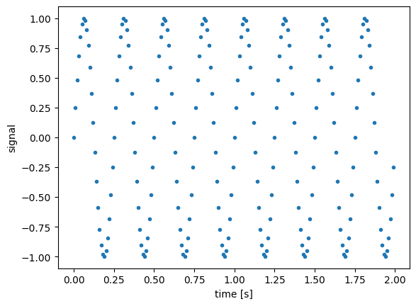
a) One Frequency#
f = 4 # frequency (Hz)
f_s = 100 # sampling rate (per second)
t_min = 0 # in seconds
t_max = 2.0
t_num = int((t_max - t_min) * f_s)
t = np.linspace(t_min, t_max, t_num, endpoint=False)
signal = np.sin(f * 2.0 * np.pi * t)
plt.figure(1)
plt.plot(t, signal, marker='.', linestyle='none')
plt.xlabel('time [s]')
plt.ylabel('signal')
plt.show()
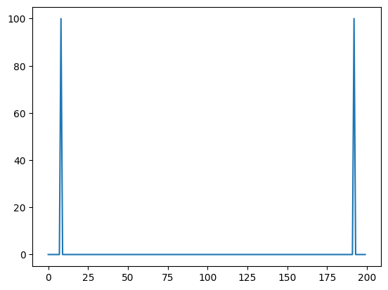
# get spectrum via discrete Fourier transform
spect = fft.fft(signal)
#print(spect)
plt.plot(np.abs(spect))
[<matplotlib.lines.Line2D at 0x7fe0501f3b60>]
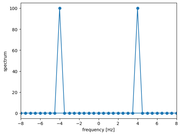
# get discrete Fourier transform sample frequencies
freqs = fft.fftfreq(n=len(signal), d=1.0/f_s)
print(freqs)
[ 0. 0.5 1. 1.5 2. 2.5 3. 3.5 4. 4.5 5. 5.5
6. 6.5 7. 7.5 8. 8.5 9. 9.5 10. 10.5 11. 11.5
12. 12.5 13. 13.5 14. 14.5 15. 15.5 16. 16.5 17. 17.5
18. 18.5 19. 19.5 20. 20.5 21. 21.5 22. 22.5 23. 23.5
24. 24.5 25. 25.5 26. 26.5 27. 27.5 28. 28.5 29. 29.5
30. 30.5 31. 31.5 32. 32.5 33. 33.5 34. 34.5 35. 35.5
36. 36.5 37. 37.5 38. 38.5 39. 39.5 40. 40.5 41. 41.5
42. 42.5 43. 43.5 44. 44.5 45. 45.5 46. 46.5 47. 47.5
48. 48.5 49. 49.5 -50. -49.5 -49. -48.5 -48. -47.5 -47. -46.5
-46. -45.5 -45. -44.5 -44. -43.5 -43. -42.5 -42. -41.5 -41. -40.5
-40. -39.5 -39. -38.5 -38. -37.5 -37. -36.5 -36. -35.5 -35. -34.5
-34. -33.5 -33. -32.5 -32. -31.5 -31. -30.5 -30. -29.5 -29. -28.5
-28. -27.5 -27. -26.5 -26. -25.5 -25. -24.5 -24. -23.5 -23. -22.5
-22. -21.5 -21. -20.5 -20. -19.5 -19. -18.5 -18. -17.5 -17. -16.5
-16. -15.5 -15. -14.5 -14. -13.5 -13. -12.5 -12. -11.5 -11. -10.5
-10. -9.5 -9. -8.5 -8. -7.5 -7. -6.5 -6. -5.5 -5. -4.5
-4. -3.5 -3. -2.5 -2. -1.5 -1. -0.5]
# plot it
plt.figure(1)
plt.plot(freqs, np.abs(spect), 'o-')
plt.xlabel('frequency [Hz]')
plt.ylabel('spectrum')
plt.xlim([-8, 8])
plt.show()
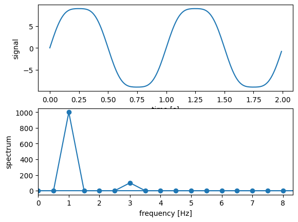
b) Two Frequencies#
f1 = 1 # frequency (Hz)
f2 = 3
f_s = 100 # sampling rate (per second)
t_min = 0 # in seconds
t_max = 2.0
t_num = int((t_max - t_min) * f_s)
t = np.linspace(t_min, t_max, t_num, endpoint=False)
#x = np.sin(f1 * 2.0 * np.pi * t) + \
# np.sin(f2 * 2.0 * np.pi * t)
x = 10 * np.sin(f1 * 2.0 * np.pi * t) + \
np.sin(f2 * 2.0 * np.pi * t)
# get spectrum via discrete Fourier transform
spect = fft.fft(x)
# get discrete Fourier transform sample frequencies
freqs = fft.fftfreq(n=len(x), d=1.0/f_s)
plt.figure(1)
plt.subplot(211)
plt.plot(t, x)
plt.xlabel('time [s]')
plt.ylabel('signal')
plt.subplot(212)
plt.plot(freqs, np.abs(spect), 'o-')
plt.xlabel('frequency [Hz]')
plt.ylabel('spectrum')
plt.xlim([0, f_s/12.0])
plt.show()
f_s = 1000 # sampling rate (per second)
t_min = 0 # in seconds
t_max = 500.0
t_num = int((t_max - t_min) * f_s)
t = np.linspace(t_min, t_max, t_num, endpoint=False)
x = np.sin(t) + 10.0*np.cos(0.1*t)
# get spectrum via discrete Fourier transform
spect = fft.fft(x)
# get discrete Fourier transform sample frequencies
freqs = fft.fftfreq(n=len(x), d=1.0/f_s)
plt.figure(1)
plt.subplot(211)
plt.plot(t, x)
plt.xlabel('time [s]')
plt.ylabel('signal')
plt.subplot(212)
plt.grid(True)
plt.plot(freqs, np.abs(spect))
#plt.yscale('log')
plt.xlabel('frequency [Hz]')
plt.ylabel('spectrum')
plt.xlim([0, 0.25])
plt.show()
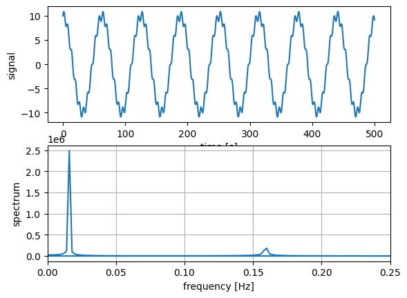
Get first frequency
print( freqs[ spect[ :int(t_num/2) ].argmax() ] )
print(0.1/(2.*np.pi))
0.016
0.015915494309189534
And the second:
spect[spect[:int(t_num/2)].argmax()] = 0
print( freqs[spect[:int(t_num/2)].argmax()] , 1./(2.*np.pi))
0.158 0.15915494309189535
Fourier Transforms 1D – Audio Spectra#
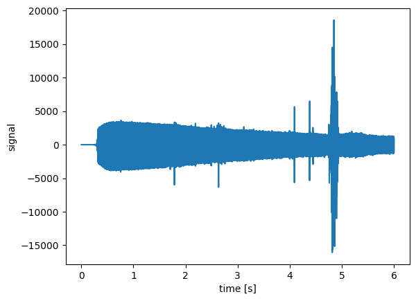
a) Sound Files – Monotonous#
from scipy.io import wavfile
from IPython.display import Audio
# open player
Audio('data/06_sounds/rec_01.wav')
---------------------------------------------------------------------------
ValueError Traceback (most recent call last)
Cell In[10], line 5
2 from IPython.display import Audio
4 # open player
----> 5 Audio('data/06_sounds/rec_01.wav')
File /usr/local/lib/python3.14/site-packages/IPython/lib/display.py:129, in Audio.__init__(self, data, filename, url, embed, rate, autoplay, normalize, element_id)
127 if self.data is not None and not isinstance(self.data, bytes):
128 if rate is None:
--> 129 raise ValueError("rate must be specified when data is a numpy array or list of audio samples.")
130 self.data = Audio._make_wav(data, rate, normalize)
ValueError: rate must be specified when data is a numpy array or list of audio samples.
# read in wavfile as data
rate, audio = wavfile.read('data/06_sounds/rec_01.wav')
# get length in seconds
N = audio.shape[0]
L = N / rate
print("Audio rate: ", rate)
print("Audio length:", L, "seconds")
plt.figure(1)
plt.plot(np.arange(N) / rate, audio)
plt.xlabel('time [s]')
plt.ylabel('signal')
plt.show()
Audio('data/06_sounds/rec_01.wav')
Audio rate: 16000
Audio length: 6.0 seconds
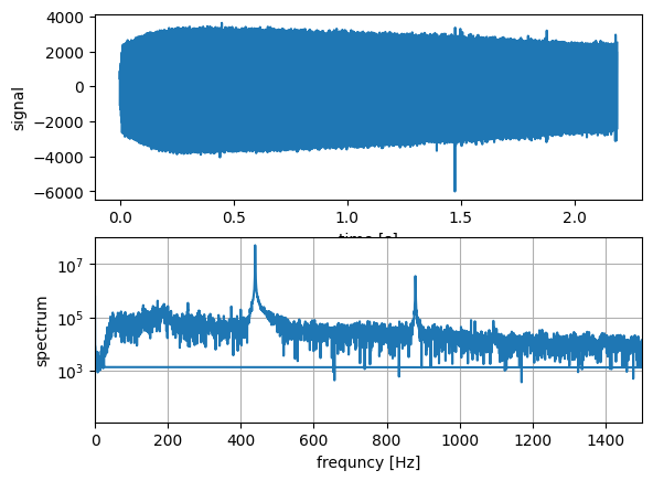
# decide which part to take
#audioSlice = audio
#audioSlice = audio[10000:20000]
#audioSlice = audio[5000:60000]
audioSlice = audio[5000:40000]
#audioSlice = audio[9000:10000]
N = np.size(audioSlice)
# get spectrum via discrete Fourier transform
spect = fft.fft(audioSlice)
# get discrete Fourier transform sample frequencies
freqs = fft.fftfreq(n=len(audioSlice), d=1.0/rate)
plt.figure(1)
plt.subplot(211)
plt.plot(np.arange(N) / rate, audioSlice)
plt.xlabel('time [s]')
plt.ylabel('signal')
plt.subplot(212)
plt.grid(True)
plt.plot(freqs, np.abs(spect))
plt.yscale('log')
plt.xlabel('frequncy [Hz]')
plt.ylabel('spectrum')
plt.xlim([0, 1500.0])
plt.show()
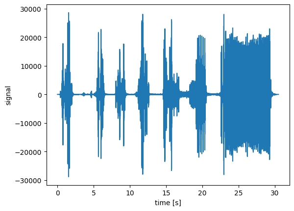
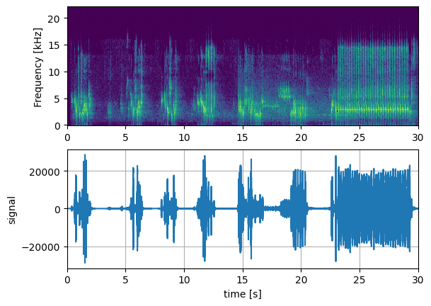
b) Sound Files – Spectrogram: Visualizing the singing bird#
# read in wavfile as data
# from http://www.orangefreesounds.com
rate, audio = wavfile.read('data/06_sounds/rec_02.wav')
# make stereo to mono
audio = np.mean(audio, axis=1)
# get length in seconds
N = audio.shape[0]
L = N / rate
print("Audio rate: ", rate)
print("Audio length:", L, "seconds")
plt.figure(1)
plt.plot(np.arange(N) / rate, audio)
plt.xlabel('time [s]')
plt.ylabel('signal')
plt.show()
Audio('data/06_sounds/rec_02.wav')
Audio rate: 44100
Audio length: 30.511020408163265 seconds
# usig scipy's signal package to create spectrogram
from scipy import signal
# read in wavfile as data
rate, audio = wavfile.read('data/06_sounds/rec_02.wav')
# make stero to mono
audio = np.mean(audio, axis=1)
freqs, times, Sx = signal.spectrogram(audio, fs=rate)
plt.figure(1)
plt.subplot(211)
plt.pcolormesh(times,
freqs / 1000,
10 * np.log(np.abs(Sx)+0.0001),
cmap='viridis')
plt.ylabel('Frequency [kHz]')
plt.xlim([0, 30])
plt.subplot(212)
plt.grid(True)
plt.plot(np.arange(N) / rate,
audio)
plt.xlabel('time [s]')
plt.ylabel('signal')
plt.xlim([0, 30])
plt.show()
Audio('data/06_sounds/rec_02.wav')
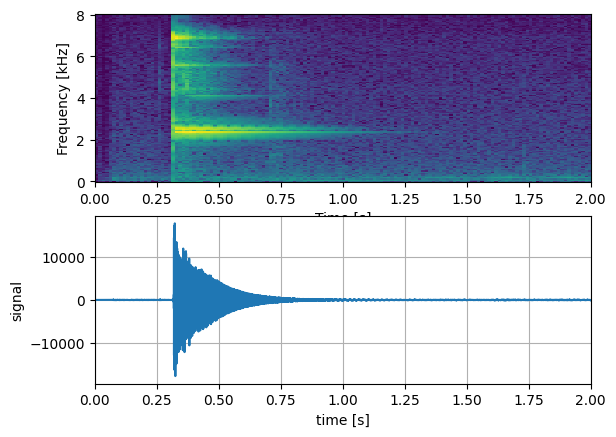
c) Sound Files – Spectrogram: Finding specific sounds#
# read in wavfile as data
rate, audio = wavfile.read('data/06_sounds/rec_03.wav')
audio = audio[4000:]
# get length in seconds
N = audio.shape[0]
L = N / rate
freqs, times, Sx = signal.spectrogram(audio, fs=rate)
plt.figure(1)
plt.subplot(211)
plt.pcolormesh(times, freqs / 1000,
10 * np.log(np.abs(Sx)+0.0001), cmap='viridis')
plt.xlabel('Time [s]')
plt.ylabel('Frequency [kHz]')
plt.xlim([0, 2.0])
plt.subplot(212)
plt.grid(True)
plt.plot(np.arange(N) / rate, audio)
plt.xlabel('time [s]')
plt.ylabel('signal')
plt.xlim([0, 2.0])
plt.show()
Audio('data/06_sounds/rec_03.wav')
# read in wavfile as data
file = 'data/06_sounds/rec_04.wav'
rate, audio = wavfile.read(file)
Audio(file)
# get length in seconds
N = audio.shape[0]
L = N / rate
freqs, times, Sx = signal.spectrogram(audio, fs=rate)
plt.figure(1)
plt.subplot(211)
plt.pcolormesh(times,
freqs / 1000,
10 * np.log(np.abs(Sx)+0.0001),
cmap='viridis')
plt.ylabel('Frequency [kHz]')
plt.subplot(212)
plt.grid(True)
plt.plot(np.arange(N) / rate, audio)
plt.xlabel('time [s]')
plt.ylabel('signal')
plt.show()
Audio(file)
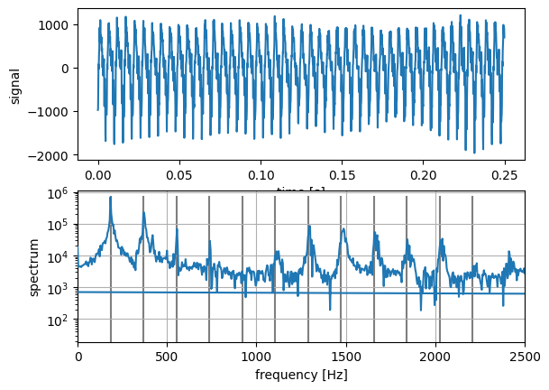
d) Sound Files – Spectrogram vs. full spectrum: Overtones#
# read in wavfile as data
file = 'data/06_sounds/rec_06.wav'
rate, audio = wavfile.read(file)
Audio(file)
#audioSlice = audio
audioSlice = audio[55000:57000, 0]
# get length in seconds
N = len(audioSlice)
L = N / rate
# get spectrum via discrete Fourier transform
spect = fft.fft(audioSlice)
# get discrete Fourier transform sample frequencies
freqs = fft.fftfreq(n=len(audioSlice), d=1.0/rate)
plt.figure(1)
plt.subplot(211)
plt.plot(np.arange(N) / rate, audioSlice)
plt.xlabel('time [s]')
plt.ylabel('signal')
plt.subplot(212)
plt.grid(True)
plt.plot(freqs, np.abs(spect), zorder=3)
plt.yscale('log')
plt.xlabel('frequency [Hz]')
plt.ylabel('spectrum')
plt.xlim([0, 2500])
# mark all overtones
freq0 = freqs[np.argmax(np.abs(spect))]
for i in range(0, 13):
plt.plot([freq0*i, freq0*i],
[0, np.max(np.abs(spect))],
zorder=1, color='tab:grey')
plt.show()
Audio(file)
freqs, times, Sx = signal.spectrogram(audio[:,0], fs=rate)
plt.figure(1)
plt.pcolormesh(times,
freqs / 1000, 10 * np.log(np.abs(Sx)+0.0001),
cmap='viridis')
plt.xlabel('Time [s]')
plt.ylabel('Frequency [kHz]')
plt.show()
Audio(file)
Fourier Transforms 1D – Fourier Filter#
a) 1D Fourier Filter: Stick to a base frequency#
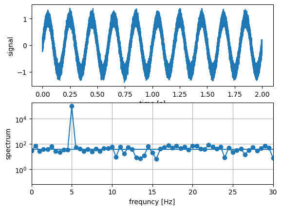
f = 5 # frequency (Hz)
f_s = 100000 # sampling rate (per second)
t_min = 0 # in seconds
t_max = 2.0
t_num = int((t_max - t_min) * f_s)
t = np.linspace(t_min, t_max, t_num, endpoint=False)
x = np.sin(f * 2.0 * np.pi * t) + 0.1*np.random.randn(t_num)
#x = np.sin(f * 2.0 * np.pi * t) + 1.0*np.random.randn(t_num)
#x = np.sin(f * 2.0 * np.pi * t) + 5.0*np.random.randn(t_num)
# get spectrum via discrete Fourier transform
spect = fft.fft(x)
# get discrete Fourier transform sample frequencies
freqs = fft.fftfreq(n=len(x), d=1.0/f_s)
plt.figure(1)
plt.subplot(211)
plt.plot(t, x)
plt.xlabel('time [s]')
plt.ylabel('signal')
plt.subplot(212)
plt.grid(True)
plt.plot(freqs, np.abs(spect), 'o-')
plt.yscale('log')
plt.xlabel('frequncy [Hz]')
plt.ylabel('spectrum')
plt.xlim([0, 30.0])
plt.show()
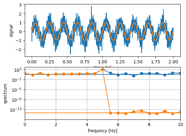
f = 5 # frequency (Hz)
f_s = 1000 # sampling rate (per second)
t_min = 0 # in seconds
t_max = 2.0
t_num = int((t_max - t_min) * f_s)
t = np.linspace(t_min, t_max, t_num, endpoint=False)
x = np.sin(f * 2.0 * np.pi * t) + 0.5*np.random.randn(t_num)
# get spectrum via discrete Fourier transform
spect = fft.fft(x)
# get discrete Fourier transform sample frequencies
freqs = fft.fftfreq(n=len(x), d=1.0/f_s)
# Remove all frequencies above peakFreq
spectFiltered = spect.copy()
peakFreq = freqs[ np.argmax(np.abs(spect)) ]
spectFiltered[ np.abs(freqs) > peakFreq ] = 0.0
# reconstruct filtered signal via inverse-FFT
xFiltered = fft.ifft(spectFiltered)
spectFiltered = fft.fft(xFiltered)
plt.figure(1)
plt.subplot(211)
plt.plot(t, x)
plt.plot(t, xFiltered, lw=2.0)
plt.xlabel('time [s]')
plt.ylabel('signal')
plt.subplot(212)
plt.grid(True)
plt.plot(freqs, np.abs(spect), 'o-')
plt.plot(freqs, np.abs(spectFiltered), 'o-')
plt.yscale('log')
plt.xlabel('frequncy [Hz]')
plt.ylabel('spectrum')
plt.xlim([0, 10.0])
plt.show()
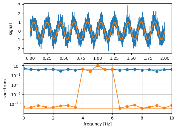
f = 5 # frequency (Hz)
f_s = 1000 # sampling rate (per second)
t_min = 0 # in seconds
t_max = 2.0
t_num = int((t_max - t_min) * f_s)
t = np.linspace(t_min, t_max, t_num, endpoint=False)
x = np.sin(f * 2.0 * np.pi * t) + 0.5*np.random.randn(t_num)
# get spectrum via discrete Fourier transform
spect = fft.fft(x)
# get discrete Fourier transform sample frequencies
freqs = fft.fftfreq(n=len(x), d=1.0/f_s)
# Remove all frequencies except for a certain window
spectFiltered = spect.copy()
peakFreq = freqs[ np.argmax(np.abs(spect)) ]
spectFiltered[ np.abs(np.abs(freqs)-peakFreq) > 1.0 ] = 0.0
# reconstruct filtered signal via inverse-FFT
xFiltered = fft.ifft(spectFiltered)
spectFiltered = fft.fft(xFiltered)
plt.figure(1)
plt.subplot(211)
plt.plot(t, x)
plt.plot(t, xFiltered, lw=2.0)
plt.xlabel('time [s]')
plt.ylabel('signal')
plt.subplot(212)
plt.grid(True)
plt.plot(freqs, np.abs(spect), 'o-')
plt.plot(freqs, np.abs(spectFiltered), 'o-')
plt.yscale('log')
plt.xlabel('frequncy [Hz]')
plt.ylabel('spectrum')
plt.xlim([0, 10.0])
plt.show()
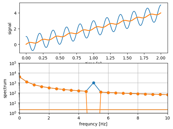
b) 1D Fourier Filter: Remove a base frequency#
f = 5 # frequency (Hz)
f_s = 1000 # sampling rate (per second)
t_min = 0 # in seconds
t_max = 2.0
t_num = int((t_max - t_min) * f_s)
t = np.linspace(t_min, t_max, t_num, endpoint=False)
x = 2.0 * t + np.cos(f * 2.0 * np.pi * t)
# get spectrum via discrete Fourier transform
spect = fft.fft(x)
# get discrete Fourier transform sample frequencies
freqs = fft.fftfreq(n=len(x), d=1.0/f_s)
# Remove the base frequency
spectFiltered = spect.copy()
peakFreq = freqs[ np.argmax(np.abs(spect)) ]
spectFiltered[ np.abs(freqs) == f ] = 0.0
# reconstruct filtered signal via inver-FFT
xFiltered = fft.ifft(spectFiltered)
spectFiltered = fft.fft(xFiltered)
plt.figure(1)
plt.subplot(211)
plt.plot(t, x)
plt.plot(t, xFiltered, lw=2.0)
plt.xlabel('time [s]')
plt.ylabel('signal')
plt.subplot(212)
plt.grid(True)
plt.plot(freqs, np.abs(spect), 'o-')
plt.plot(freqs, np.abs(spectFiltered), 'o-')
plt.yscale('log')
plt.xlabel('frequncy [Hz]')
plt.ylabel('spectrum')
plt.xlim([0, 10.0])
plt.ylim([0.9, 100000.0])
plt.show()
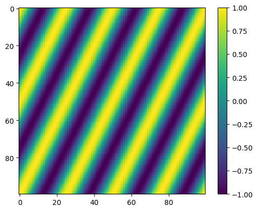
Fourier Transforms 2D#
# create 2D data and plot it
N = 100
def f2D(x, y):
fx = 2
fy = 4
return np.cos((fx * x + fy * y) * 2.0 * np.pi / N)
data2D = np.fromfunction(f2D, (N, N))
plt.figure(1)
plt.clf()
plt.imshow(data2D)
plt.colorbar()
plt.show()
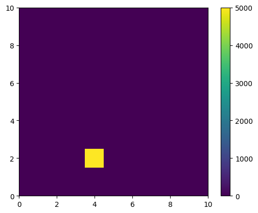
spect2D = fft.fftn(data2D)
plt.figure(1)
plt.clf()
plt.imshow(np.abs(spect2D))
plt.xlim([0, 10])
plt.ylim([0, 10])
plt.colorbar()
plt.show()
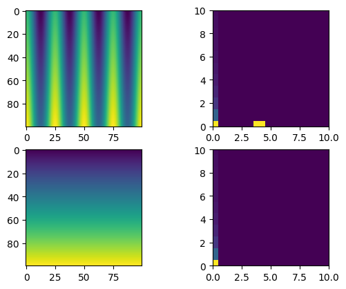
Fourier Transforms 2D – Fourier Filter#
a) Simple Example#
# create 2D data and plot it
N = 100
def f2D(x, y):
f = 4.0
return x + 100.0*np.cos(f * (y) * 2.0 * np.pi / N)
# get original 2D data
data2D = np.fromfunction(f2D, (N, N))
spect2D = fft.fftn(data2D)
# generate filtered data
spect2DFiltered = spect2D.copy()
spect2DFiltered[:,2:] = np.zeros((N,N-2))
data2DFiltered = fft.ifftn(spect2DFiltered)
plt.figure(1)
plt.subplot(221)
plt.imshow(data2D)
plt.subplot(222)
plt.imshow(np.abs(spect2D))
plt.xlim([0, 10])
plt.ylim([0, 10])
plt.subplot(223)
plt.imshow(np.abs(data2DFiltered))
plt.subplot(224)
plt.imshow(np.abs(spect2DFiltered))
plt.xlim([0, 10])
plt.ylim([0, 10])
plt.show()
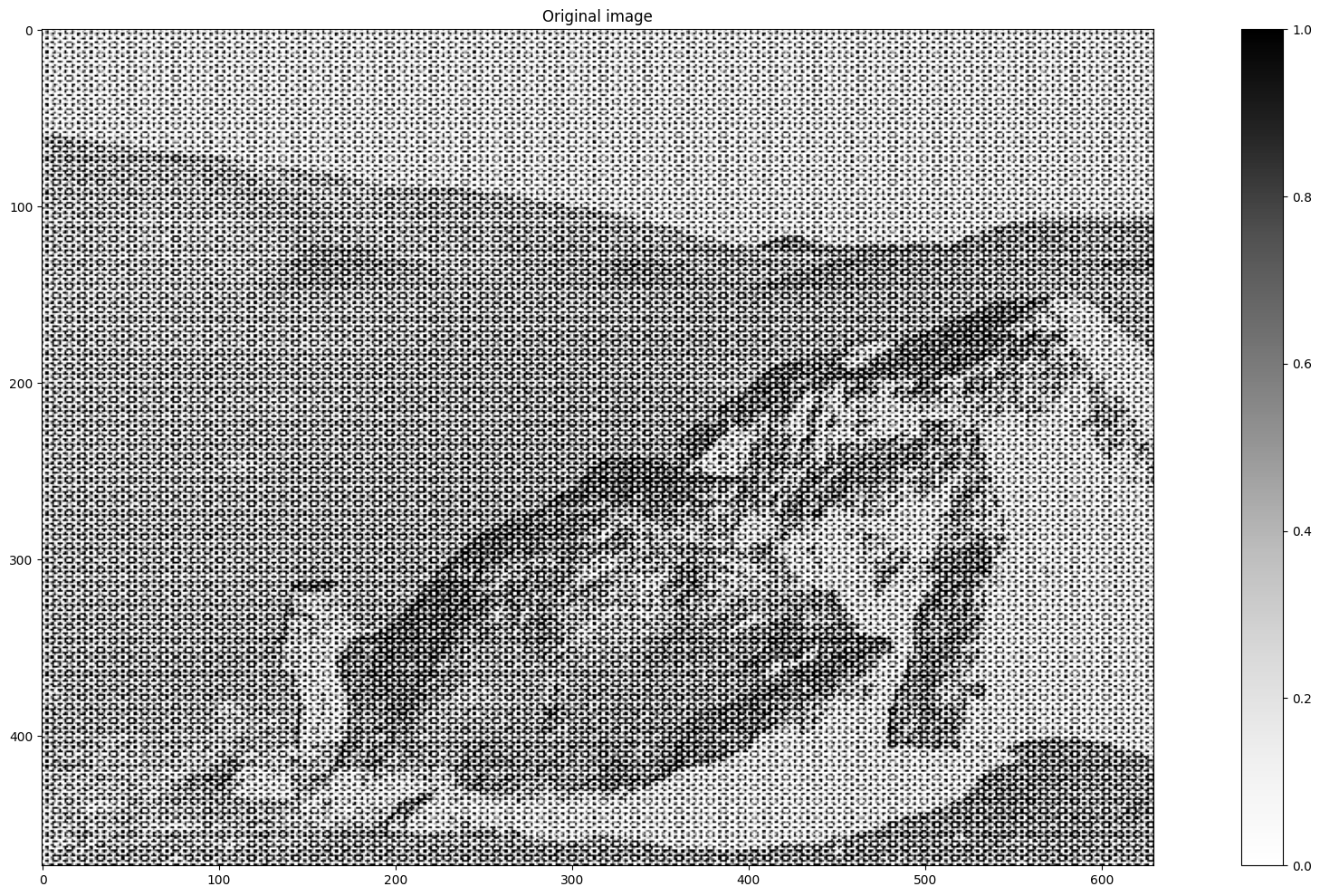
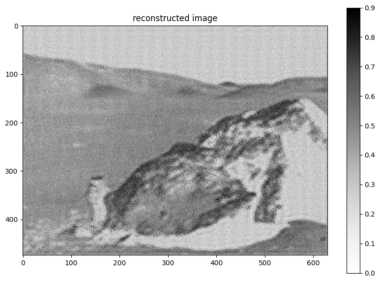
b) Simple 2D FT Filter: Application to actual images#
# use imread to read in image
image = plt.imread('data/07_moonlanding.png').astype(float)
M, N = image.shape
plt.figure(1, figsize=(25, 12))
plt.imshow(image, cmap='Greys')
plt.colorbar()
plt.title('Original image')
plt.show()
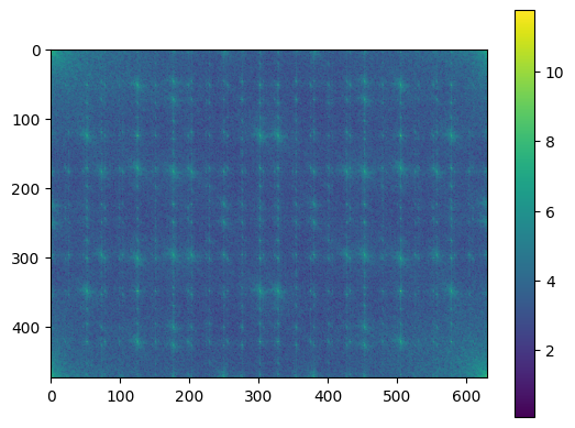
# vizualize 2d spectrum
spect = fft.fftn(image)
plt.figure(1)
plt.imshow(np.log(1+np.abs(spect)))
plt.colorbar()
plt.show()
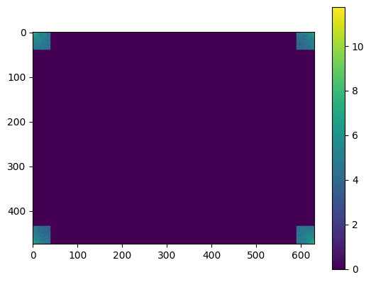
# apply brute-force-filter and mask everything excepts the corners
k = 40
spectFiltered = np.zeros((M, N), dtype=complex)
spectFiltered[0:k, 0:k] = spect[0:k, 0:k]
spectFiltered[0:k, N-k:N] = spect[0:k, N-k:N]
spectFiltered[M-k:M, 0:k] = spect[M-k:M, 0:k]
spectFiltered[M-k:M, N-k:N] = spect[M-k:M, N-k:N]
plt.figure(1)
plt.imshow(np.log(1+np.abs(spectFiltered)))
plt.colorbar()
plt.show()
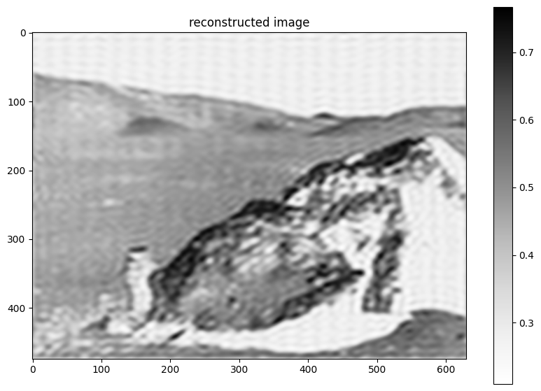
plt.figure(2, figsize=(10, 7))
plt.imshow(np.real(fft.ifftn(spectFiltered)), cmap='Greys')
plt.colorbar()
plt.title('reconstructed image')
plt.show()
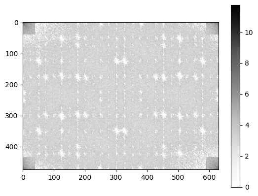
# apply masking filter
spectFiltered = spect.copy()
k = 40
spectMag = np.abs(spect.copy())
spectMag[0:k, 0:k] = 0.0
spectMag[0:k, N-k:N] = 0.0
spectMag[M-k:M, 0:k] = 0.0
spectMag[M-k:M, N-k:N] = 0.0
spectFiltered = spect.copy()
spectFiltered[spectMag > np.max(spectMag)*0.002] = 0.0
plt.figure(1)
plt.imshow(np.log(1+np.abs(spectFiltered)), cmap='Greys')
plt.colorbar()
plt.show()
plt.figure(2, figsize=(10, 7))
plt.imshow(np.real(fft.ifftn(spectFiltered)),
cmap='Greys', vmin=0.0, vmax=0.9)
plt.colorbar()
plt.title('reconstructed image')
plt.show()
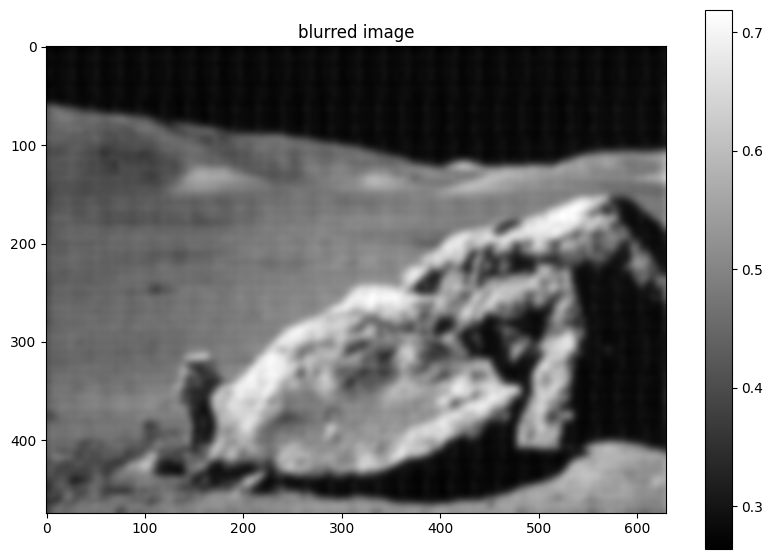
# easier ... via Gaussian smearing
from scipy import ndimage
im_blur = ndimage.gaussian_filter(image, 4)
plt.figure(1, figsize=(10, 7))
plt.imshow(im_blur, plt.cm.gray)
plt.colorbar()
plt.title('blurred image')
plt.show()