Random Numbers

---

Start with NumPy and matplotlib:

import numpy as np
import matplotlib.pylab as plt

Random Number Generation

Get a random number via NumPy’s random module, using its rand() function:

a = np.random.rand()

print( a )

0.7672451703800369

Get a whole random matrix:

A = np.random.rand(3, 3, 2)

print( A )

[[[0.99227986 0.30622325]
  [0.30131488 0.59967493]
  [0.63837998 0.54534001]]

 [[0.62730555 0.94456943]
  [0.55941718 0.71779347]
  [0.46527538 0.45750565]]

 [[0.37142985 0.87645323]
  [0.3180609  0.80357048]
  [0.24840259 0.15517278]]]

True vs. Pseudo Random Numbers

Computer algorithms commonly create pseudo random numbers with “good” statistics, but being dependent on a seed:

... 93802948542771471902796694497278419429380485689050661139408044323 ...
         | start here ...                     | or here ... 

in NumPy we can set the seed on our own:

np.random.seed(29)

a = np.random.rand()
print( a )

0.8637599855700829

which will set the whole series of following random numbers:

np.random.seed(29)

a = np.random.rand()
print( a )

a = np.random.rand()
print( a )

a = np.random.rand()
print( a )

0.8637599855700829
0.2849059652276268
0.07325638808373602

Note

Seeding can be handy to test algorithms using random numbers!

Different Statistics

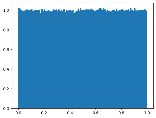
np.random.rand(): Uniform distribution

Get a random vector and plot its histogram:

N = 1000000
b = np.random.rand(N)

plt.figure(1)
plt.hist(b, bins=100, density=True)
plt.show()

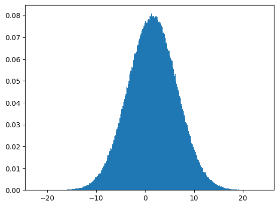
np.random.normal(): Normal (Gaussian) distribution

N = 1000000
b = np.random.normal(size=N, loc=1.5, scale=5.0)

plt.figure(1)
plt.hist(b, bins=300, density=True)
plt.show()

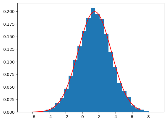
#?np.random.normal

def gauss(mu, sigma, x):
    return 1/(sigma * np.sqrt(2 * np.pi)) \
           * np.exp( - (x - mu)**2 / (2 * sigma**2) )

plt.figure(1)

b = np.random.normal(size=10000, loc=1.5, scale=2.0)
plt.hist(b, bins=30, density=True)

xPlot = np.linspace(-7, 7, 100)
plt.plot(xPlot, gauss(mu=1.5, sigma=2.0, x=xPlot), 'r-')

plt.show()

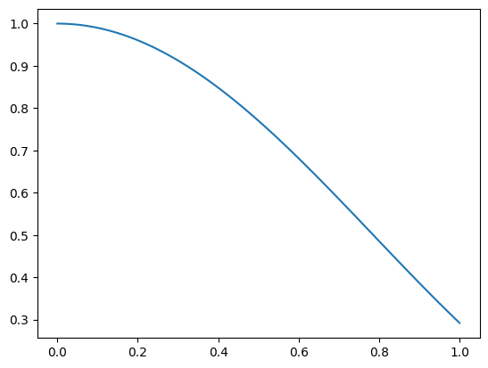
Integration via Random Numbers / Coordinates

\[ A = \int_0^1 cos^2(x) \, dx\]

def f(x):
    return np.cos(x)**2.0

xFine = np.linspace(0, 1, 100)

plt.figure(1)
plt.plot(xFine, f(xFine))
plt.show()

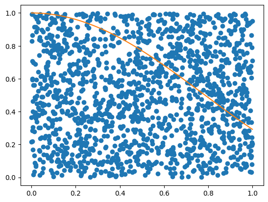
Get random x and y coordinates:

low = [0,0]
high = [1,1]
points = np.random.uniform(low ,high, size=(1500,2))
x, y = points[:,0], points[:,1]

plt.figure(1)
plt.plot(x, y, 'o')
plt.plot(xFine, f(xFine))
plt.show()

Now mark points below and above f(x):

indAbove = np.where( y >= f(x)  )[0]
indBelow = np.where( y < f(x) )[0]

plt.figure(1)
plt.plot(x[indAbove], y[indAbove], 'o')
plt.plot(x[indBelow], y[indBelow], 'o')
plt.plot(xFine, f(xFine))
plt.show()

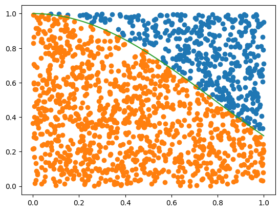
Finally get an estimate of the integral of f(x) from 0 to 1 by comparing the amount of points below f(x) to the total number of points and compare to SciPy’s quad():

intRand = len(indBelow) / ( len(indBelow) + len(indAbove) )

print("Monte Carlo:", intRand )

import scipy.integrate as integrate
intQuad, error = integrate.quad(f, a=0, b=1)

print("      SciPy:", intQuad )

Monte Carlo: 0.7193333333333334

      SciPy: 0.7273243567064205

Multi-Dimensional Integration via Random Numbers / Coordinates

\[ A = \int_{0}^{2} \int_{0}^{2} \frac{ e^{-x\,t} }{t^2 + 1} \, dx \, dt\]

def f(x,t):
    return np.exp(-x*t) / (t**2 + 1)

# get random numbers
N = 1500
x, t = np.random.rand(2, N) * 2.0
y    = np.random.rand(N, N) * 2.0

# get the volume of the FULL space we have been sampling
volume = 2.0 * 2.0 * 2.0

# create a meshgrid of our random (x,t) coordinates
# so that we can call f(xGrid, tGrid)
xGrid, tGrid = np.meshgrid(x, t)

# count how often our random y(x,t) lays below f(x,t)
indBelow = np.where( y <= f(xGrid, tGrid) )

# and calculate the interal with the proper normalization!
intRand = len(indBelow[0]) * volume / N**2.0

# multi-dimensional integral via scipy's integrate.nquad
intQuad, error = integrate.nquad(f, [[0, 2],
                                     [0, 2]])

print("Monte Carlo:", intRand )
print("      SciPy:", intQuad )

Monte Carlo: 1.2833422222222222
      SciPy: 1.3039147247360718

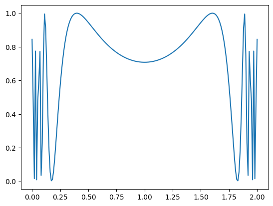
Mean Values via Random Numbers

\[ \bar{f} = \frac{1}{b-a} \int_a^b f(x) dx \]

for $\( f(x) = sin \left( \frac{ 1 }{x(2-x)} \right)^2, \)\( which is problematic for \)a=0\( and \)b=2$.

# define a function f(x) we like to consider
def f(x):
    return (np.sin(1/(x*(2-x))))**2

N = 200
x = np.linspace(0.0001, 1.9999, N)
y = f(x)

plt.figure(1)
plt.plot(x, y)
plt.show()

#?integrate.quad

d = 0.1
a = 0 + d
b = 2 -d

intQuad, error = integrate.quad(f, a=a, b=b)
print( 1/(b-a) * intQuad )

0.7550327874373094

Let’s calculate the standard mean for a variety of starting points x0:

N = 10000
for x0 in np.logspace(-1, -6, 8):
    
    print( "%f : %f"%(x0, f(np.linspace(x0, 1, N)).mean() ))

0.100000 : 0.755029
0.019307 : 0.729971
0.003728 : 0.726605
0.000720 : 0.725740
0.000139 : 0.726149
0.000027 : 0.725691
0.000005 : 0.725232
0.000001 : 0.725425

And for a variety of N:

for N in range(100000, 1000000, 100000):
    
    print( "%d : %f"%(N, f(2.0 * np.random.rand(N)).mean()))

100000 : 0.725837
200000 : 0.726622
300000 : 0.725721
400000 : 0.726297
500000 : 0.725663
600000 : 0.725421
700000 : 0.725388
800000 : 0.725737

900000 : 0.726596

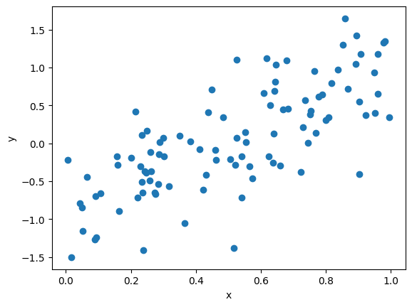
Simulating an Experiment via Random Numbers

N = 100
# create x on a random grid
x = np.random.rand(N)

# and y = 2.0 * x - 1.0 
# ... and add Gaussian noise (like in an experiment) to it
y = 2.0 * x - 1.0 + np.random.normal(scale=0.5, size=N)

# and plot everything
plt.figure(1)
plt.plot(x, y, 'o')
plt.xlabel('x')
plt.ylabel('y')
plt.show()

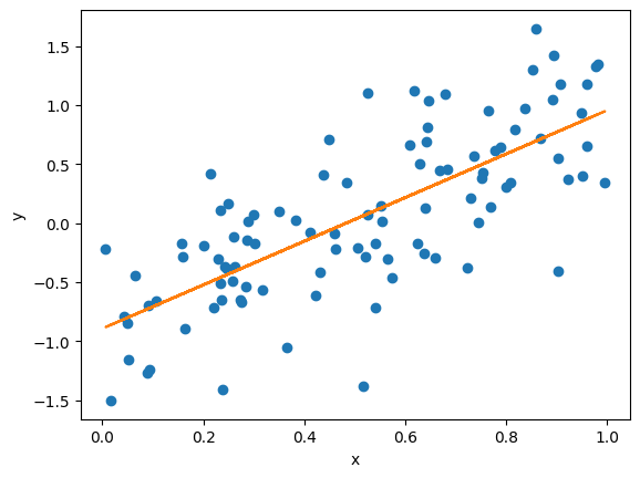
# load curve_fit from scipy
from scipy.optimize import curve_fit

# define a linear function
def fitFunc(x, a, b):
    return a * x + b

# and fit it to the noisy data
myFit, V = curve_fit(fitFunc, x, y)

# get error estimate
error = np.sqrt(np.diag(V))  

# print out fitting parameters
print(" a = %+4.3f +/- %4.3f"%(myFit[0], error[0]))
print(" b = %+4.3f +/- %4.3f"%(myFit[1], error[1]))

# and plot everything
plt.figure(1)
plt.plot(x, y, 'o')
plt.plot(x, fitFunc(x, *myFit))
plt.xlabel('x')
plt.ylabel('y')
plt.show()

 a = +1.848 +/- 0.168
 b = -0.893 +/- 0.099

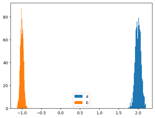
# let's have a look into the STATISTICS of our fitting parameters

N     = 1000          # Number of random sets ... for the statistics
a     = np.zeros(N)   # array to save all fitted a 
b     = np.zeros(N)   # array to save all fitted a 

# loop over sets
for i in range(N):
    
    # create a new set
    x = np.random.rand(50)
    y = 2.0 * x - 1.0 + np.random.normal(scale=0.15, size=50)
    
    # and fit it to the noisy data
    myFit, V = curve_fit(fitFunc, x, y)
    
    # get error estimate
    error = np.sqrt(np.diag(V))  

    # save a and b
    a[i] = myFit[0]
    b[i] = myFit[1]
    
#plt.subplot(2, 1, 1)
plt.hist(a, bins=int(np.sqrt(N)), label='$a$' )
plt.hist(b, bins=int(np.sqrt(N)), label='$b$' )
plt.legend() 

#plt.subplot(2,1,2)
#plt.hist(b, bins=int(np.sqrt(N)), label='$b$' )
#plt.legend() 

plt.show()

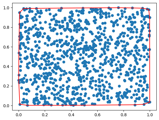
Convex hull of a square

# function that returns all points of A (set of x/y points)
# which belong to its convex hull
def getHull(A):
    
    N = np.size(A[:,0])
    
    # create an empty list of corner indices
    ind = []

    # add the top-most (largest y position) point to the list of corner indices
    # ... since it belongs to our convex hull by definition
    ind.append( np.argmax(A[:,1]) )

    # initial values for our search
    lastAngle  = -4.0
    closed     = False

    # search for all points of the convex hull via while loop
    # ... continue the search as long as the hull is not closed
    while (not closed):
        
        # Algorithm idea: find the next point with smallest angle 
        #                 larger than previous angle

        # generate a list of angles between our last point and all other points
        newAngles = np.arctan2(A[:, 1] - A[ind[-1], 1], 
                               A[:, 0] - A[ind[-1], 0])
        
        # "penalty" for angle = 0
        newAngles[np.where(newAngles == 0)] += 1000.0
        
        # find the smallest angle from our "penalized" angle list
        nextInd = np.argmin(np.abs(lastAngle - newAngles))

        # check if the next index is already in our list
        if(nextInd in ind):
            # ... if yes the hull is closed
            closed = True
            
        else:
            # ... if not we save the angle between the last and the next
            #            angle as our "lastAngle"
            lastAngle = np.arctan2(A[nextInd,1] - A[ind[-1],1],
                                   A[nextInd,0] - A[ind[-1],0])
            
            # and add the nextIndex to the list of our hull array
            ind.append( nextInd )
            
    return ind


# generate N random (x,y)
N = 1000
A = np.random.rand(N, 2)

# and plot them
plt.plot(A[:,0], A[:,1], 'o')

ind = getHull(A)
    
# plot line connecting all corner indices
for ii in range(np.size(ind)):
    plt.plot( A[[ind[ii-1], ind[ii]], 0],
              A[[ind[ii-1], ind[ii]], 1], 'r')
    
plt.show()

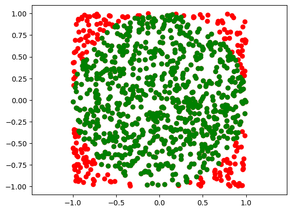
Convex hull of a circle

# generate N random (x,y)
N = 1000
A = np.random.rand(N, 2) * 2.0 - 1.0

# get all points which belong to a circle of with radius = 1
ind = np.where( np.sqrt( A[:,0]**2.0 + A[:,1]**2.0) <= 1 )[0]

# and plot them
plt.plot(A[:,0], A[:,1], 'or')
plt.plot(A[ind,0], A[ind,1], 'og')
plt.axis('equal')
plt.show()

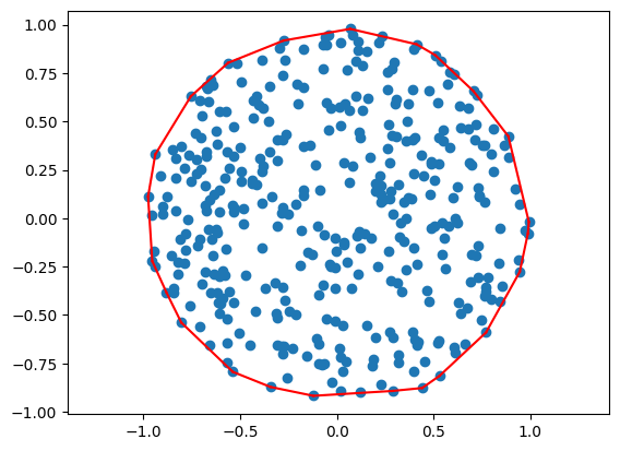
# generate N random (x,y)
N = 500
A = np.random.rand(N, 2) * 2.0 - 1.0

ind = np.where( np.sqrt( A[:,0]**2.0 + A[:,1]**2.0) <= 1 )[0]

# and plot them
plt.plot(A[ind,0], A[ind,1], 'o')

circle = A[ind,:]

ind = getHull(circle)
    
# plot line connecting all corner indices
for ii in range(np.size(ind)):
    plt.plot( circle[[ind[ii-1], ind[ii]], 0],
              circle[[ind[ii-1], ind[ii]], 1], 'r')
    
plt.axis('equal') 
plt.show()